
16.16: Countercurrent Separations
- Page ID
- 135883

\( \newcommand{\vecs}[1]{\overset { \scriptstyle \rightharpoonup} {\mathbf{#1}} } \)
\( \newcommand{\vecd}[1]{\overset{-\!-\!\rightharpoonup}{\vphantom{a}\smash {#1}}} \)
\( \newcommand{\dsum}{\displaystyle\sum\limits} \)
\( \newcommand{\dint}{\displaystyle\int\limits} \)
\( \newcommand{\dlim}{\displaystyle\lim\limits} \)
\( \newcommand{\id}{\mathrm{id}}\) \( \newcommand{\Span}{\mathrm{span}}\)
( \newcommand{\kernel}{\mathrm{null}\,}\) \( \newcommand{\range}{\mathrm{range}\,}\)
\( \newcommand{\RealPart}{\mathrm{Re}}\) \( \newcommand{\ImaginaryPart}{\mathrm{Im}}\)
\( \newcommand{\Argument}{\mathrm{Arg}}\) \( \newcommand{\norm}[1]{\| #1 \|}\)
\( \newcommand{\inner}[2]{\langle #1, #2 \rangle}\)
\( \newcommand{\Span}{\mathrm{span}}\)
\( \newcommand{\id}{\mathrm{id}}\)
\( \newcommand{\Span}{\mathrm{span}}\)
\( \newcommand{\kernel}{\mathrm{null}\,}\)
\( \newcommand{\range}{\mathrm{range}\,}\)
\( \newcommand{\RealPart}{\mathrm{Re}}\)
\( \newcommand{\ImaginaryPart}{\mathrm{Im}}\)
\( \newcommand{\Argument}{\mathrm{Arg}}\)
\( \newcommand{\norm}[1]{\| #1 \|}\)
\( \newcommand{\inner}[2]{\langle #1, #2 \rangle}\)
\( \newcommand{\Span}{\mathrm{span}}\) \( \newcommand{\AA}{\unicode[.8,0]{x212B}}\)
\( \newcommand{\vectorA}[1]{\vec{#1}} % arrow\)
\( \newcommand{\vectorAt}[1]{\vec{\text{#1}}} % arrow\)
\( \newcommand{\vectorB}[1]{\overset { \scriptstyle \rightharpoonup} {\mathbf{#1}} } \)
\( \newcommand{\vectorC}[1]{\textbf{#1}} \)
\( \newcommand{\vectorD}[1]{\overrightarrow{#1}} \)
\( \newcommand{\vectorDt}[1]{\overrightarrow{\text{#1}}} \)
\( \newcommand{\vectE}[1]{\overset{-\!-\!\rightharpoonup}{\vphantom{a}\smash{\mathbf {#1}}}} \)
\( \newcommand{\vecs}[1]{\overset { \scriptstyle \rightharpoonup} {\mathbf{#1}} } \)
\(\newcommand{\longvect}{\overrightarrow}\)
\( \newcommand{\vecd}[1]{\overset{-\!-\!\rightharpoonup}{\vphantom{a}\smash {#1}}} \)
\(\newcommand{\avec}{\mathbf a}\) \(\newcommand{\bvec}{\mathbf b}\) \(\newcommand{\cvec}{\mathbf c}\) \(\newcommand{\dvec}{\mathbf d}\) \(\newcommand{\dtil}{\widetilde{\mathbf d}}\) \(\newcommand{\evec}{\mathbf e}\) \(\newcommand{\fvec}{\mathbf f}\) \(\newcommand{\nvec}{\mathbf n}\) \(\newcommand{\pvec}{\mathbf p}\) \(\newcommand{\qvec}{\mathbf q}\) \(\newcommand{\svec}{\mathbf s}\) \(\newcommand{\tvec}{\mathbf t}\) \(\newcommand{\uvec}{\mathbf u}\) \(\newcommand{\vvec}{\mathbf v}\) \(\newcommand{\wvec}{\mathbf w}\) \(\newcommand{\xvec}{\mathbf x}\) \(\newcommand{\yvec}{\mathbf y}\) \(\newcommand{\zvec}{\mathbf z}\) \(\newcommand{\rvec}{\mathbf r}\) \(\newcommand{\mvec}{\mathbf m}\) \(\newcommand{\zerovec}{\mathbf 0}\) \(\newcommand{\onevec}{\mathbf 1}\) \(\newcommand{\real}{\mathbb R}\) \(\newcommand{\twovec}[2]{\left[\begin{array}{r}#1 \\ #2 \end{array}\right]}\) \(\newcommand{\ctwovec}[2]{\left[\begin{array}{c}#1 \\ #2 \end{array}\right]}\) \(\newcommand{\threevec}[3]{\left[\begin{array}{r}#1 \\ #2 \\ #3 \end{array}\right]}\) \(\newcommand{\cthreevec}[3]{\left[\begin{array}{c}#1 \\ #2 \\ #3 \end{array}\right]}\) \(\newcommand{\fourvec}[4]{\left[\begin{array}{r}#1 \\ #2 \\ #3 \\ #4 \end{array}\right]}\) \(\newcommand{\cfourvec}[4]{\left[\begin{array}{c}#1 \\ #2 \\ #3 \\ #4 \end{array}\right]}\) \(\newcommand{\fivevec}[5]{\left[\begin{array}{r}#1 \\ #2 \\ #3 \\ #4 \\ #5 \\ \end{array}\right]}\) \(\newcommand{\cfivevec}[5]{\left[\begin{array}{c}#1 \\ #2 \\ #3 \\ #4 \\ #5 \\ \end{array}\right]}\) \(\newcommand{\mattwo}[4]{\left[\begin{array}{rr}#1 \amp #2 \\ #3 \amp #4 \\ \end{array}\right]}\) \(\newcommand{\laspan}[1]{\text{Span}\{#1\}}\) \(\newcommand{\bcal}{\cal B}\) \(\newcommand{\ccal}{\cal C}\) \(\newcommand{\scal}{\cal S}\) \(\newcommand{\wcal}{\cal W}\) \(\newcommand{\ecal}{\cal E}\) \(\newcommand{\coords}[2]{\left\{#1\right\}_{#2}}\) \(\newcommand{\gray}[1]{\color{gray}{#1}}\) \(\newcommand{\lgray}[1]{\color{lightgray}{#1}}\) \(\newcommand{\rank}{\operatorname{rank}}\) \(\newcommand{\row}{\text{Row}}\) \(\newcommand{\col}{\text{Col}}\) \(\renewcommand{\row}{\text{Row}}\) \(\newcommand{\nul}{\text{Nul}}\) \(\newcommand{\var}{\text{Var}}\) \(\newcommand{\corr}{\text{corr}}\) \(\newcommand{\len}[1]{\left|#1\right|}\) \(\newcommand{\bbar}{\overline{\bvec}}\) \(\newcommand{\bhat}{\widehat{\bvec}}\) \(\newcommand{\bperp}{\bvec^\perp}\) \(\newcommand{\xhat}{\widehat{\xvec}}\) \(\newcommand{\vhat}{\widehat{\vvec}}\) \(\newcommand{\uhat}{\widehat{\uvec}}\) \(\newcommand{\what}{\widehat{\wvec}}\) \(\newcommand{\Sighat}{\widehat{\Sigma}}\) \(\newcommand{\lt}{<}\) \(\newcommand{\gt}{>}\) \(\newcommand{\amp}{&}\) \(\definecolor{fillinmathshade}{gray}{0.9}\)In 1949, Lyman Craig introduced an improved method for separating analytes with similar distribution ratios [Craig, L. C. J. Biol. Chem. 1944, 155, 519–534]. The technique, which is known as a countercurrent liquid–liquid extraction, is outlined in Figure 16.16.1 and discussed in detail below. In contrast to a sequential liquid–liquid extraction, in which we repeatedly extract the sample containing the analyte, a countercurrent extraction uses a serial extraction of both the sample and the extracting phases. Although countercurrent separations are no longer common—chromatographic separations are far more efficient in terms of resolution, time, and ease of use—the theory behind a countercurrent extraction remains useful as an introduction to the theory of chromatographic separations.
To track the progress of a countercurrent liquid-liquid extraction we need to adopt a labeling convention. As shown in Figure 16.16.1 , in each step of a countercurrent extraction we first complete the extraction and then transfer the upper phase to a new tube that contains a portion of the fresh lower phase. Steps are labeled sequentially beginning with zero. Extractions take place in a series of tubes that also are labeled sequentially, starting with zero. The upper and lower phases in each tube are identified by a letter and number, with the letters U and L representing, respectively, the upper phase and the lower phase, and the number indicating the step in the countercurrent extraction in which the phase was first introduced. For example, U0 is the upper phase introduced at step 0 (during the first extraction), and L2 is the lower phase introduced at step 2 (during the third extraction). Finally, the partitioning of analyte in any extraction tube results in a fraction p remaining in the upper phase, and a fraction q remaining in the lower phase. Values of q are calculated using Equation \ref{16.1}, which is identical to Equation 7.7.6 in Chapter 7.
\[(q_\text{aq})_1 = \frac {(\text{mol aq})_1} {(\text{mol aq})_0} = \frac {V_\text{aq}} {D V_\text{org} + V_\text{aq}} \label{16.1}\]
The fraction p, of course is equal to 1 – q. Typically Vaq and Vorg are equal in a countercurrent extraction, although this is not a requirement.
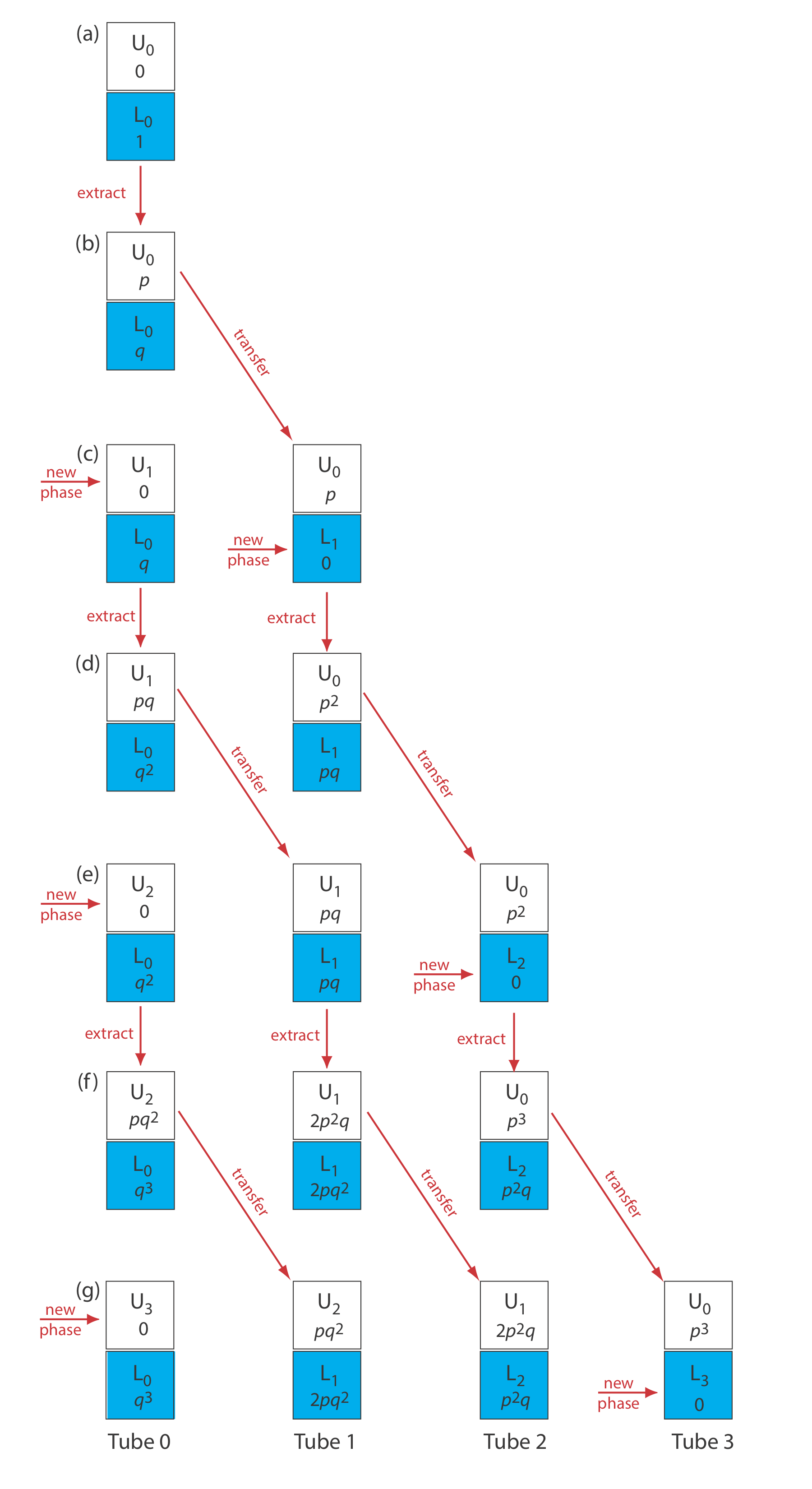
Let’s assume that the analyte we wish to isolate is present in an aqueous phase of 1 M HCl, and that the organic phase is benzene. Because benzene has the smaller density, it is the upper phase, and 1 M HCl is the lower phase. To begin the countercurrent extraction we place the aqueous sample that contains the analyte in tube 0 along with an equal volume of benzene. As shown in Figure \(\PageIndex{1}\text{a}\), before the extraction all the analyte is present in phase L0. When the extraction is complete, as shown in Figure \(\PageIndex{1}\text{b}\), a fraction p of the analyte is present in phase U0, and a fraction q is in phase L0. This completes step 0 of the countercurrent extraction. If we stop here, there is no difference between a simple liquid–liquid extraction and a countercurrent extraction.
After completing step 0, we remove phase U0 and add a fresh portion of benzene, U1, to tube 0 (see Figure \(\PageIndex{1}\text{c}\)). This, too, is identical to a simple liquid-liquid extraction. Here is where the power of the countercurrent extraction begins—instead of setting aside the phase U0, we place it in tube 1 along with a portion of analyte-free aqueous 1 M HCl as phase L1 (see Figure \(\PageIndex{1}\text{c}\)). Tube 0 now contains a fraction q of the analyte, and tube 1 contains a fraction p of the analyte. Completing the extraction in tube 0 results in a fraction p of its contents remaining in the upper phase, and a fraction q remaining in the lower phase. Thus, phases U1 and L0 now contain, respectively, fractions pq and q2 of the original amount of analyte. Following the same logic, it is easy to show that the phases U0 and L1 in tube 1 contain, respectively, fractions p2 and pq of analyte. This completes step 1 of the extraction (see Figure \(\PageIndex{1}\text{d}\)). As shown in the remainder of Figure 16.16.1 , the countercurrent extraction continues with this cycle of phase transfers and extractions.
In a countercurrent liquid–liquid extraction, the lower phase in each tube remains in place, and the upper phase moves from tube 0 to successively higher numbered tubes. We recognize this difference in the movement of the two phases by referring to the lower phase as a stationary phase and the upper phase as a mobile phase. With each transfer some of the analyte in tube r moves to tube \(r + 1\), while a portion of the analyte in tube \(r - 1\) moves to tube r. Analyte introduced at tube 0 moves with the mobile phase, but at a rate that is slower than the mobile phase because, at each step, a portion of the analyte transfers into the stationary phase. An analyte that preferentially extracts into the stationary phase spends proportionally less time in the mobile phase and moves at a slower rate. As the number of steps increases, analytes with different values of q eventually separate into completely different sets of extraction tubes.
We can judge the effectiveness of a countercurrent extraction using a histogram that shows the fraction of analyte present in each tube. To determine the total amount of analyte in an extraction tube we add together the fraction of analyte present in the tube’s upper and lower phases following each transfer. For example, at the beginning of step 3 (see Figure \(\PageIndex{1}\text{g}\)) the upper and lower phases of tube 1 contain fractions pq2 and 2pq2 of the analyte, respectively; thus, the total fraction of analyte in the tube is 3pq2. Table 16.16.1 summarizes this for the steps outlined in Figure 16.16.1 . A typical histogram, calculated assuming distribution ratios of 5.0 for analyte A and 0.5 for analyte B, is shown in Figure 16.16.2 . Although four steps is not enough to separate the analytes in this instance, it is clear that if we extend the countercurrent extraction to additional tubes, we will eventually separate the analytes.
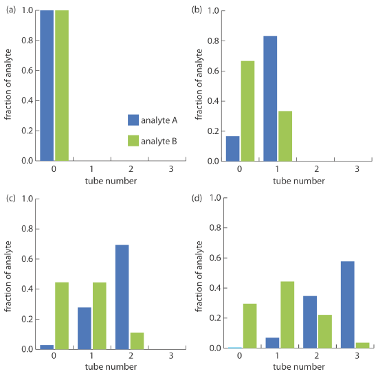
Figure 16.16.1 and Table 16.16.1 show how an analyte’s distribution changes during the first four steps of a countercurrent extraction. Now we consider how we can generalize these results to calculate the amount of analyte in any tube, at any step during the extraction. You may recognize the pattern of entries in Table 16.16.1 as following the binomial distribution
\[f(r, n) = \frac {n!} {(n - r)! r!} p^{r} q^{n - r} \label{16.2}\]
where f(r, n) is the fraction of analyte present in tube r at step n of the countercurrent extraction, with the upper phase containing a fraction \(p \times f(r, n)\) of analyte and the lower phase containing a fraction \(q \times f(r, n)\) of the analyte.
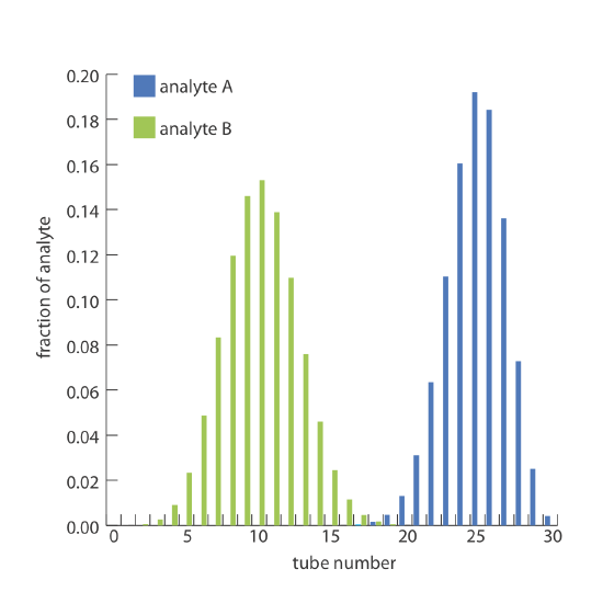
The countercurrent extraction shown in Figure 16.16.2 is carried out through step 30. Calculate the fraction of analytes A and B in tubes 5, 10, 15, 20, 25, and 30.
Solution
To calculate the fraction, q, for each analyte in the lower phase we use Equation \ref{16.1}. Because the volumes of the lower and upper phases are equal, we get
\[q_\text{A} = \frac {1} {D_\text{A} + 1} = \frac {1} {5 + 1} = 0.167 \quad \quad q_\text{B} = \frac {1} {D_\text{B} + 1} = \frac {1} {0.5 + 1} = 0.667 \nonumber\]
Because we know that \(p + q = 1 \), we also know that pA is 0.833 and that pB is 0.333. For analyte A, the fraction in tubes 5, 10, 15, 20, 25, and 30 after the 30th step are
\[f(5,30) = \frac {30!} {(30 - 5)! 5!} (0.833)^{5} (0.167)^{30 - 5} = 2.1 \times 10^{-15} \approx 0 \nonumber\]
\[f(10,30) = \frac {30!} {(30 - 10)! 10!} (0.833)^{10} (0.167)^{30 - 10} = 1.4 \times 10^{-9} \approx 0 \nonumber\]
\[f(15,30) = \frac {30!} {(30 - 15)! 5!} (0.833)^{15} (0.167)^{30 - 15} = 2.2 \times 10^{-5} \approx 0 \nonumber\]
\[f(20,30) = \frac {30!} {(30 - 20)! 20!} (0.833)^{20} (0.167)^{30 - 20} = 0.013 \nonumber\]
\[f(25,30) = \frac {30!} {(30 - 25)! 25!} (0.833)^{25} (0.167)^{30 - 25} = 0.192 \nonumber\]
\[f(30,30) = \frac {30!} {(30 - 30)! 30!} (0.833)^{30} (0.167)^{30 - 30} = 0.004 \nonumber\]
The fraction of analyte B in tubes 5, 10, 15, 20, 25, and 30 is calculated in the same way, yielding respective values of 0.023, 0.153, 0.025, 0, 0, and 0. Figure 16.16.3 , which provides the complete histogram for the distribution of analytes A and B, shows that 30 steps is sufficient to separate the two analytes.
Constructing a histogram using Equation \ref{16.2} is tedious, particularly when the number of steps is large. Because the fraction of analyte in most tubes is approximately zero, we can simplify the histogram’s construction by solving Equation \ref{16.2} only for those tubes containing an amount of analyte that exceeds a threshold value. For a binomial distribution, we can use the mean and standard deviation to determine which tubes contain a significant fraction of analyte. The properties of a binomial distribution were covered in Chapter 4, with the mean, \(\mu\), and the standard deviation, \(\sigma\), given as
\[\mu = np \nonumber\]
\[\sigma = \sqrt{np(1 - p)} = \sqrt{npq} \nonumber\]
Furthermore, if both np and nq are greater than 5, then a binomial distribution closely approximates a normal distribution and we can use the properties of a normal distribution to determine the location of the analyte and its recovery [see Mark, H.; Workman, J. Spectroscopy 1990, 5(3), 55–56].
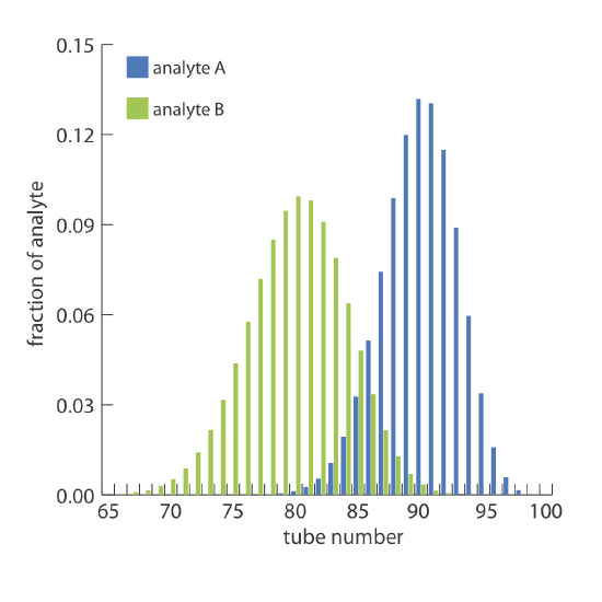
Two analytes, A and B, with distribution ratios of 9 and 4, respectively, are separated using a countercurrent extraction in which the volumes of the upper and lower phases are equal. After 100 steps determine the 99% confidence interval for the location of each analyte.
Solution
The fraction, q, of each analyte that remains in the lower phase is calculated using Equation \ref{16.1}. Because the volumes of the lower and upper phases are equal, we find that
\[q_\text{A} = \frac {1} {D_\text{A} + 1} = \frac {1} {9 + 1} = 0.10 \quad \quad q_\text{B} = \frac {1} {D_\text{B} + 1} = \frac {1} {4 + 1} = 0.20 \nonumber\]
Because we know that \(p + q = 1 \), we also know that pA is 0.90 and pB is 0.80. After 100 steps, the mean and the standard deviation for the distribution of analytes A and B are
\[\mu_\text{A} = np_\text{A} = (100)(0.90) = 90 \text{ and } \sigma_\text{A} = \sqrt{np_\text{A}q_\text{A}} = \sqrt{(100)(0.90)(0.10)} = 3 \nonumber\]
\[\mu_\text{B} = np_\text{B} = (100)(0.80) = 80 \text{ and } \sigma_\text{A} = \sqrt{np_\text{A}q_\text{A}} = \sqrt{(100)(0.80)(0.20)} = 4 \nonumber\]
Given that npA, npB, nqA, and nqB are all greater than 5, we can assume that the distribution of analytes follows a normal distribution and that the confidence interval for the tubes containing each analyte is
\[r = \mu \pm z \sigma \nonumber\]
where r is the tube’s number and the value of z is determined by the desired significance level. For a 99% confidence interval the value of z is 2.58 (see Appendix 4); thus,
\[r_\text{A} = 90 \pm (2.58)(3) = 90 \pm 8 \nonumber\]
\[r_\text{B} = 80 \pm (2.58)(4) = 80 \pm 10 \nonumber\]
Because the two confidence intervals overlap, a complete separation of the two analytes is not possible using a 100 step countercurrent extraction. The complete distribution of the analytes is shown in Figure 16.16.4 .
For the countercurrent extraction in Example 16.16.2 , calculate the recovery and the separation factor for analyte A if the contents of tubes 85–99 are pooled together.
Solution
From Example 16.16.2 we know that after 100 steps of the countercurrent extraction, analyte A is normally distributed about tube 90 with a standard deviation of 3. To determine the fraction of analyte A in tubes 85–99, we use the single-sided normal distribution in Appendix 3 to determine the fraction of analyte in tubes 0–84, and in tube 100. The fraction of analyte A in tube 100 is determined by calculating the deviation z
\[z = \frac {r - \mu} {\sigma} = \frac {99 - 90} {3} = 3 \nonumber\]
and using the table in Appendix 3 to determine the corresponding fraction. For z = 3 this corresponds to 0.135% of analyte A. To determine the fraction of analyte A in tubes 0–84 we again calculate the deviation
\[z = \frac {r - \mu} {\sigma} = \frac {84 - 90} {3} = -1.67 \nonumber\]
From Appendix 3 we find that 4.75% of analyte A is present in tubes 0–84. Analyte A’s recovery, therefore, is
\[100\% - 4.75\% - 0.135\% \approx 95\% \nonumber\]
To calculate the separation factor we determine the recovery of analyte B in tubes 85–99 using the same general approach as for analyte A, finding that approximately 89.4% of analyte B remains in tubes 0–84 and that essentially no analyte B is in tube 100. The recovery for B, therefore, is
\[100\% - 89.4\% - 0\% \approx 10.6\% \nonumber\]
and the separation factor is
\[S_\text{B/A} = \frac {R_\text{A}} {R_\text{B}} = \frac {10.6} {95} = 0.112 \nonumber\]