
11.1: Overview of Electrochemistry
- Page ID
- 154796

\( \newcommand{\vecs}[1]{\overset { \scriptstyle \rightharpoonup} {\mathbf{#1}} } \)
\( \newcommand{\vecd}[1]{\overset{-\!-\!\rightharpoonup}{\vphantom{a}\smash {#1}}} \)
\( \newcommand{\dsum}{\displaystyle\sum\limits} \)
\( \newcommand{\dint}{\displaystyle\int\limits} \)
\( \newcommand{\dlim}{\displaystyle\lim\limits} \)
\( \newcommand{\id}{\mathrm{id}}\) \( \newcommand{\Span}{\mathrm{span}}\)
( \newcommand{\kernel}{\mathrm{null}\,}\) \( \newcommand{\range}{\mathrm{range}\,}\)
\( \newcommand{\RealPart}{\mathrm{Re}}\) \( \newcommand{\ImaginaryPart}{\mathrm{Im}}\)
\( \newcommand{\Argument}{\mathrm{Arg}}\) \( \newcommand{\norm}[1]{\| #1 \|}\)
\( \newcommand{\inner}[2]{\langle #1, #2 \rangle}\)
\( \newcommand{\Span}{\mathrm{span}}\)
\( \newcommand{\id}{\mathrm{id}}\)
\( \newcommand{\Span}{\mathrm{span}}\)
\( \newcommand{\kernel}{\mathrm{null}\,}\)
\( \newcommand{\range}{\mathrm{range}\,}\)
\( \newcommand{\RealPart}{\mathrm{Re}}\)
\( \newcommand{\ImaginaryPart}{\mathrm{Im}}\)
\( \newcommand{\Argument}{\mathrm{Arg}}\)
\( \newcommand{\norm}[1]{\| #1 \|}\)
\( \newcommand{\inner}[2]{\langle #1, #2 \rangle}\)
\( \newcommand{\Span}{\mathrm{span}}\) \( \newcommand{\AA}{\unicode[.8,0]{x212B}}\)
\( \newcommand{\vectorA}[1]{\vec{#1}} % arrow\)
\( \newcommand{\vectorAt}[1]{\vec{\text{#1}}} % arrow\)
\( \newcommand{\vectorB}[1]{\overset { \scriptstyle \rightharpoonup} {\mathbf{#1}} } \)
\( \newcommand{\vectorC}[1]{\textbf{#1}} \)
\( \newcommand{\vectorD}[1]{\overrightarrow{#1}} \)
\( \newcommand{\vectorDt}[1]{\overrightarrow{\text{#1}}} \)
\( \newcommand{\vectE}[1]{\overset{-\!-\!\rightharpoonup}{\vphantom{a}\smash{\mathbf {#1}}}} \)
\( \newcommand{\vecs}[1]{\overset { \scriptstyle \rightharpoonup} {\mathbf{#1}} } \)
\(\newcommand{\longvect}{\overrightarrow}\)
\( \newcommand{\vecd}[1]{\overset{-\!-\!\rightharpoonup}{\vphantom{a}\smash {#1}}} \)
\(\newcommand{\avec}{\mathbf a}\) \(\newcommand{\bvec}{\mathbf b}\) \(\newcommand{\cvec}{\mathbf c}\) \(\newcommand{\dvec}{\mathbf d}\) \(\newcommand{\dtil}{\widetilde{\mathbf d}}\) \(\newcommand{\evec}{\mathbf e}\) \(\newcommand{\fvec}{\mathbf f}\) \(\newcommand{\nvec}{\mathbf n}\) \(\newcommand{\pvec}{\mathbf p}\) \(\newcommand{\qvec}{\mathbf q}\) \(\newcommand{\svec}{\mathbf s}\) \(\newcommand{\tvec}{\mathbf t}\) \(\newcommand{\uvec}{\mathbf u}\) \(\newcommand{\vvec}{\mathbf v}\) \(\newcommand{\wvec}{\mathbf w}\) \(\newcommand{\xvec}{\mathbf x}\) \(\newcommand{\yvec}{\mathbf y}\) \(\newcommand{\zvec}{\mathbf z}\) \(\newcommand{\rvec}{\mathbf r}\) \(\newcommand{\mvec}{\mathbf m}\) \(\newcommand{\zerovec}{\mathbf 0}\) \(\newcommand{\onevec}{\mathbf 1}\) \(\newcommand{\real}{\mathbb R}\) \(\newcommand{\twovec}[2]{\left[\begin{array}{r}#1 \\ #2 \end{array}\right]}\) \(\newcommand{\ctwovec}[2]{\left[\begin{array}{c}#1 \\ #2 \end{array}\right]}\) \(\newcommand{\threevec}[3]{\left[\begin{array}{r}#1 \\ #2 \\ #3 \end{array}\right]}\) \(\newcommand{\cthreevec}[3]{\left[\begin{array}{c}#1 \\ #2 \\ #3 \end{array}\right]}\) \(\newcommand{\fourvec}[4]{\left[\begin{array}{r}#1 \\ #2 \\ #3 \\ #4 \end{array}\right]}\) \(\newcommand{\cfourvec}[4]{\left[\begin{array}{c}#1 \\ #2 \\ #3 \\ #4 \end{array}\right]}\) \(\newcommand{\fivevec}[5]{\left[\begin{array}{r}#1 \\ #2 \\ #3 \\ #4 \\ #5 \\ \end{array}\right]}\) \(\newcommand{\cfivevec}[5]{\left[\begin{array}{c}#1 \\ #2 \\ #3 \\ #4 \\ #5 \\ \end{array}\right]}\) \(\newcommand{\mattwo}[4]{\left[\begin{array}{rr}#1 \amp #2 \\ #3 \amp #4 \\ \end{array}\right]}\) \(\newcommand{\laspan}[1]{\text{Span}\{#1\}}\) \(\newcommand{\bcal}{\cal B}\) \(\newcommand{\ccal}{\cal C}\) \(\newcommand{\scal}{\cal S}\) \(\newcommand{\wcal}{\cal W}\) \(\newcommand{\ecal}{\cal E}\) \(\newcommand{\coords}[2]{\left\{#1\right\}_{#2}}\) \(\newcommand{\gray}[1]{\color{gray}{#1}}\) \(\newcommand{\lgray}[1]{\color{lightgray}{#1}}\) \(\newcommand{\rank}{\operatorname{rank}}\) \(\newcommand{\row}{\text{Row}}\) \(\newcommand{\col}{\text{Col}}\) \(\renewcommand{\row}{\text{Row}}\) \(\newcommand{\nul}{\text{Nul}}\) \(\newcommand{\var}{\text{Var}}\) \(\newcommand{\corr}{\text{corr}}\) \(\newcommand{\len}[1]{\left|#1\right|}\) \(\newcommand{\bbar}{\overline{\bvec}}\) \(\newcommand{\bhat}{\widehat{\bvec}}\) \(\newcommand{\bperp}{\bvec^\perp}\) \(\newcommand{\xhat}{\widehat{\xvec}}\) \(\newcommand{\vhat}{\widehat{\vvec}}\) \(\newcommand{\uhat}{\widehat{\uvec}}\) \(\newcommand{\what}{\widehat{\wvec}}\) \(\newcommand{\Sighat}{\widehat{\Sigma}}\) \(\newcommand{\lt}{<}\) \(\newcommand{\gt}{>}\) \(\newcommand{\amp}{&}\) \(\definecolor{fillinmathshade}{gray}{0.9}\)The focus of this chapter is on analytical techniques that use a measurement of potential, current, or charge to determine an analyte’s concentration or to characterize an analyte’s chemical reactivity. Collectively we call this area of analytical chemistry electrochemistry because its originated from the study of the movement of electrons in an oxidation–reduction reaction.
Despite the difference in instrumentation, all electrochemical techniques share several common features. Before we consider individual examples in greater detail, let’s take a moment to consider some of these similarities. As you work through the chapter, this overview will help you focus on similarities between different electrochemical methods of analysis. You will find it easier to understand a new analytical method when you can see its relationship to other similar methods.
Five Important Concepts
To understand electrochemistry we need to appreciate five important and interrelated concepts: (1) the electrode’s potential determines the analyte’s form at the electrode’s surface; (2) the concentration of analyte at the electrode’s surface may not be the same as its concentration in bulk solution; (3) in addition to an oxidation–reduction reaction, the analyte may participate in other chemical reactions; (4) current is a measure of the rate of the analyte’s oxidation or reduction; and (5) we cannot control simultaneously current and potential.
The material in this section—particularly the five important concepts—draws upon a vision for understanding electrochemistry outlined by Larry Faulkner in the article “Understanding Electrochemistry: Some Distinctive Concepts,” J. Chem. Educ. 1983, 60, 262–264. See also, Kissinger, P. T.; Bott, A. W. “Electrochemistry for the Non-Electrochemist,” Current Separations, 2002, 20:2, 51–53.
The Electrode's Potential Determines the Analyte's Form
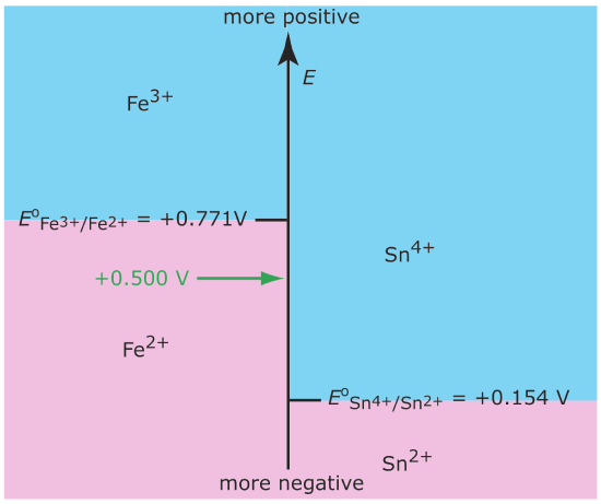
In Chapter 6 we introduced the ladder diagram as a tool for predicting how a change in solution conditions affects the position of an equilibrium reaction. Figure 11.1.1 , for example, shows a ladder diagram for the Fe3+/Fe2+ and the Sn4+/Sn2+ equilibria. If we place an electrode in a solution of Fe3+ and Sn4+ and adjust its potential to +0.500 V, Fe3+ is reduced to Fe2+ but Sn4+ is not reduced to Sn2+.
Interfacial Concentrations May Not Equal Bulk Concentrations
In Chapter 6 we introduced the Nernst equation, which provides a mathematical relationship between the electrode’s potential and the concentrations of an analyte’s oxidized and reduced forms in solution. For example, the Nernst equation for Fe3+ and Fe2+ is
\[E=E_{\mathrm{Fe}^{3+} / \mathrm{Fe}^{2+}}-\frac{R T}{n F} \ln \frac{\left[\mathrm{Fe}^{2+}\right]}{\left[\mathrm{Fe}^{3+}\right]}=\frac{0.05916}{1} \log \frac{\left[\mathrm{Fe}^{2+}\right]}{\left[\mathrm{Fe}^{3+}\right]} \label{11.1}\]
where E is the electrode’s potential and \(E_{\text{Fe}^{3+}/\text{Fe}^{2+}}^{\circ}\) is the standard-state reduction potential for the reaction \(\text{Fe}^{3+}(aq) \rightleftharpoons \text{ Fe}^{2+}(aq) + e^-\). Because it is the potential of the electrode that determines the analyte’s form at the electrode’s surface, the concentration terms in Equation \ref{11.1} are those of Fe2+ and Fe3+ at the electrode's surface, not their concentrations in bulk solution.
This distinction between a species’ surface concentration and its bulk concentration is important. Suppose we place an electrode in a solution of Fe3+ and fix its potential at 1.00 V. From the ladder diagram in Figure 11.1.1 , we know that Fe3+ is stable at this potential and, as shown in Figure 11.1.2 a, the concentration of Fe3+ is the same at all distances from the electrode’s surface. If we change the electrode’s potential to +0.500 V, the concentration of Fe3+ at the electrode’s surface decreases to approximately zero. As shown in Figure 11.1.2 b, the concentration of Fe3+ increases as we move away from the electrode’s surface until it equals the concentration of Fe3+ in bulk solution. The resulting concentration gradient causes additional Fe3+ from the bulk solution to diffuse to the electrode’s surface.
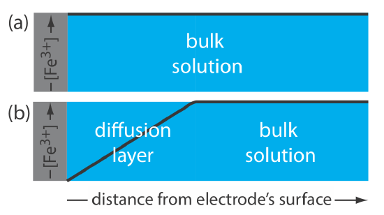
We call the region of solution that contains this concentration gradient in Fe3+ the diffusion layer. We will have more to say about this in Chapter 11.4.
The Analyte May Participate in Other Reactions
Figure 11.1.1 and Figure 11.1.2 shows how the electrode’s potential affects the concentration of Fe3+ and how the concentration of Fe3+ varies as a function of distance from the electrode’s surface. The reduction of Fe3+ to Fe2+, which is governed by Equation \ref{11.1}, may not be the only reaction that affects the concentration of Fe3+ in bulk solution or at the electrode’s surface. The adsorption of Fe3+ at the electrode’s surface or the formation of a metal–ligand complex in bulk solution, such as Fe(OH)2+, also affects the concentration of Fe3+.
Current is a Measure of Rate
The reduction of Fe3+ to Fe2+ consumes an electron, which is drawn from the electrode. The oxidation of another species, perhaps the solvent, at a second electrode is the source of this electron. Because the reduction of Fe3+ to Fe2+ consumes one electron, the flow of electrons between the electrodes—in other words, the current—is a measure of the rate at which Fe3+ is reduced. One important consequence of this observation is that the current is zero when the reaction \(\text{Fe}^{3+}(aq) \rightleftharpoons \text{ Fe}^{2+}(aq) + e^-\) is at equilibrium.
The rate of the reaction \(\text{Fe}^{3+}(aq) \rightleftharpoons \text{ Fe}^{2+}(aq) + e^-\) is the change in the concentration of Fe3+ as a function of time.
We Cannot Control Simultaneously Both the Current and the Potential
If a solution of Fe3+ and Fe2+ is at equilibrium, the current is zero and the potential is given by Equation \ref{11.1}. If we change the potential away from its equilibrium position, current flows as the system moves toward its new equilibrium position. Although the initial current is quite large, it decreases over time, reaching zero when the reaction reaches equilibrium. The current, therefore, changes in response to the applied potential. Alternatively, we can pass a fixed current through the electrochemical cell, forcing the reduction of Fe3+ to Fe2+. Because the concentrations of Fe3+ decreases and the concentration of Fe2+ increases, the potential, as given by Equation \ref{11.1}, also changes over time. In short, if we choose to control the potential, then we must accept the resulting current, and we must accept the resulting potential if we choose to control the current.
Controlling and Measuring Current and Potential
Electrochemical measurements are made in an electrochemical cell that consists of two or more electrodes and the electronic circuitry needed to control and measure the current and the potential. In this section we introduce the basic components of electrochemical instrumentation.
The simplest electrochemical cell uses two electrodes. The potential of one electrode is sensitive to the analyte’s concentration, and is called the working electrode or the indicator electrode. The second electrode, which we call the counter electrode, completes the electrical circuit and provides a reference potential against which we measure the working electrode’s potential. Ideally the counter electrode’s potential remains constant so that we can assign to the working electrode any change in the overall cell potential. If the counter electrode’s potential is not constant, then we replace it with two electrodes: a reference electrode whose potential remains constant and an auxiliary electrode that completes the electrical circuit.
Because we cannot control simultaneously the current and the potential, there are only three basic experimental designs: (1) we can measure the potential when the current is zero, (2) we can measure the potential while we control the current, and (3) we can measure the current while we control the potential. Each of these experimental designs relies on Ohm’s law, which states that the current, i, passing through an electrical circuit of resistance, R, generates a potential, E.
\[E = i R\nonumber\]
Each of these experimental designs uses a different type of instrument. To help us understand how we can control and measure current and potential, we will describe these instruments as if the analyst is operating them manually. To do so the analyst observes a change in the current or the potential and manually adjusts the instrument’s settings to maintain the desired experimental conditions. It is important to understand that modern electrochemical instruments provide an automated, electronic means for controlling and measuring current and potential, and that they do so by using very different electronic circuitry than that described here.
This point bears repeating: It is important to understand that the experimental designs in Figure 11.1.3 , Figure 11.1.4 , and Figure 11.1.5 do not represent the electrochemical instruments you will find in today’s analytical labs. For further information about modern electrochemical instrumentation, see this chapter’s additional resources.
Potentiometers
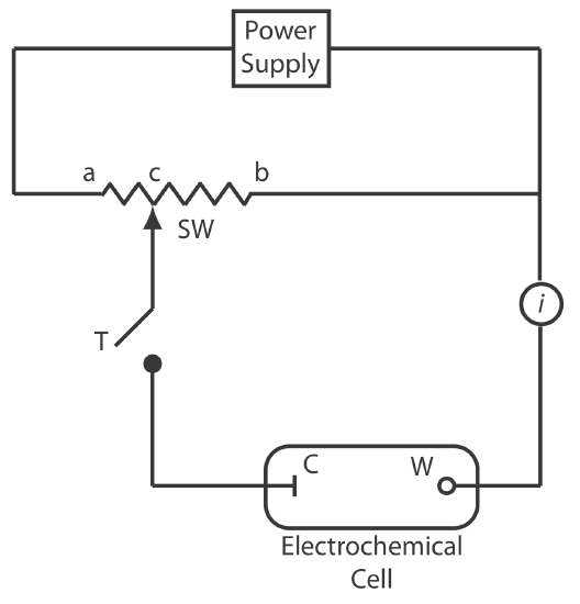
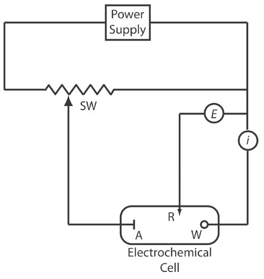
To measure the potential of an electrochemical cell under a condition of zero current we use a potentiometer. Figure 11.1.3 shows a schematic diagram for a manual potentiometer that consists of a power supply, an electrochemical cell with a working electrode and a counter electrode, an ammeter to measure the current that passes through the electrochemical cell, an adjustable, slide-wire resistor, and a tap key for closing the circuit through the electrochemical cell. Using Ohm’s law, the current in the upper half of the circuit is
\[i_{\text {upper}}=\frac{E_{\mathrm{PS}}}{R_{a b}} \nonumber\]
where EPS is the power supply’s potential, and Rab is the resistance between points a and b of the slide-wire resistor. In a similar manner, the current in the lower half of the circuit is
\[i_{\text {lower}}=\frac{E_{\text {cell}}}{R_{c b}} \nonumber\]
where Ecell is the potential difference between the working electrode and the counter electrode, and Rcb is the resistance between the points c and b of the slide-wire resistor. When iupper = ilower = 0, no current flows through the ammeter and the potential of the electrochemical cell is
\[E_{\mathrm{coll}}=\frac{R_{c b}}{R_{a b}} \times E_{\mathrm{PS}} \label{11.2}\]
To determine Ecell we briefly press the tap key and observe the current at the ammeter. If the current is not zero, then we adjust the slide wire resistor and remeasure the current, continuing this process until the current is zero. When the current is zero, we use Equation \ref{11.2} to calculate Ecell.
Using the tap key to briefly close the circuit through the electrochemical cell minimizes the current that passes through the cell and limits the change in the electrochemical cell’s composition. For example, passing a current of 10–9 A through the electrochemical cell for 1 s changes the concentrations of species in the cell by approximately 10–14 moles. Modern potentiometers use operational amplifiers to create a high-impedance voltmeter that measures the potential while drawing a current of less than 10–9 A.
Galvanostats
A galvanostat, a schematic diagram of which is shown in Figure 11.1.4 , allows us to control the current that flows through an electrochemical cell. The current from the power supply through the working electrode is
\[i=\frac{E_{\mathrm{PS}}}{R+R_{\mathrm{cell}}} \nonumber\]
where EPS is the potential of the power supply, R is the resistance of the resistor, and Rcell is the resistance of the electrochemical cell. If R >> Rcell, then the current between the auxiliary and working electrodes
\[i=\frac{E_{\mathrm{PS}}}{R} \approx \text{constant} \nonumber\]
maintains a constant value. To monitor the working electrode’s potential, which changes as the composition of the electrochemical cell changes, we can include an optional reference electrode and a high-impedance potentiometer.
Potentiostats
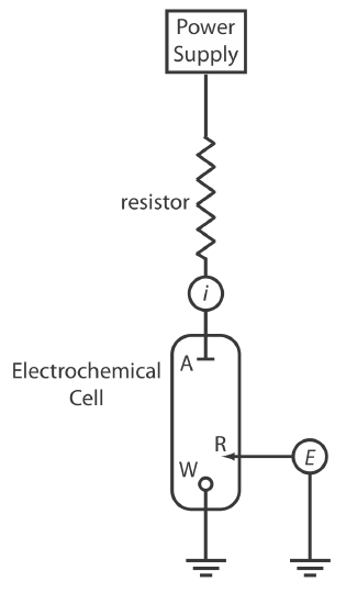
A potentiostat, a schematic diagram of which is shown in Figure 11.1.5 , allows us to control the working electrode’s potential. The potential of the working electrode is measured relative to a constant-potential reference electrode that is connected to the working electrode through a high-impedance potentiometer. To set the working electrode’s potential we adjust the slide wire resistor that is connected to the auxiliary electrode. If the working electrode’s potential begins to drift, we adjust the slide wire resistor to return the potential to its initial value. The current flowing between the auxiliary electrode and the working electrode is measured with an ammeter. Modern potentiostats include waveform generators that allow us to apply a time-dependent potential profile, such as a series of potential pulses, to the working electrode.
Interfacial Electrochemical Techniques
Because interfacial electrochemistry is such a broad field, let’s use Figure 11.1.6 to organize techniques by the experimental conditions we choose to use (Do we control the potential or the current? How do we change the applied potential or applied current? Do we stir the solution?) and the analytical signal we decide to measure (Current? Potential?).
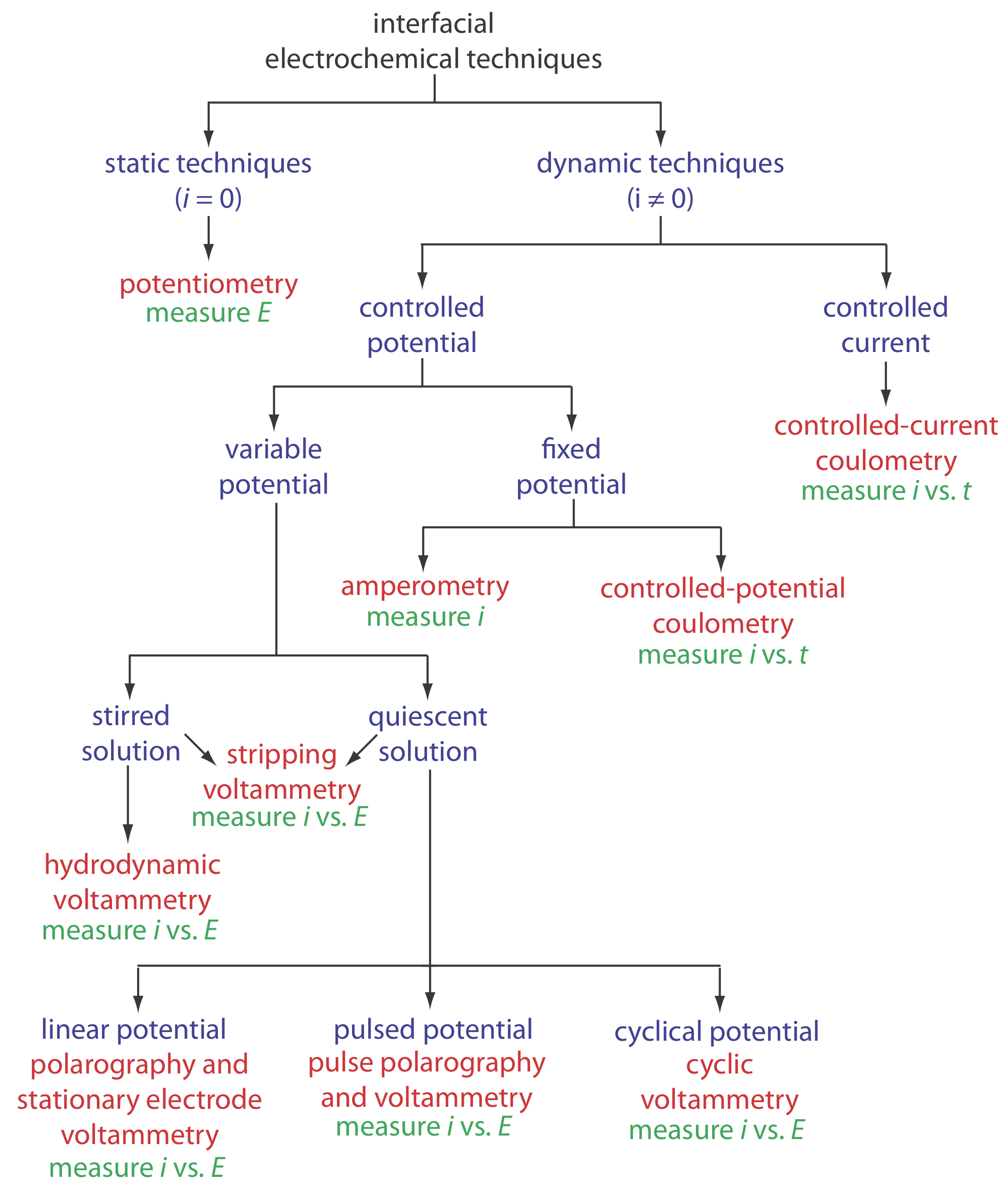
At the first level, we divide interfacial electrochemical techniques into static techniques and dynamic techniques. In a static technique we do not allow current to pass through the electrochemical cell and, as a result, the concentrations of all species remain constant. Potentiometry, in which we measure the potential of an electrochemical cell under static conditions, is one of the most important quantitative electrochemical methods and is discussed in detail in Chapter 11.2.
Dynamic techniques, in which we allow current to flow and force a change in the concentration of species in the electrochemical cell, comprise the largest group of interfacial electrochemical techniques. Coulometry, in which we measure current as a function of time, is covered in Chapter 11.3. Amperometry and voltammetry, in which we measure current as a function of a fixed or variable potential, is the subject of Chapter 11.4.