
11.4: Voltammetric and Amperometric Methods
- Page ID
- 154799

\( \newcommand{\vecs}[1]{\overset { \scriptstyle \rightharpoonup} {\mathbf{#1}} } \)
\( \newcommand{\vecd}[1]{\overset{-\!-\!\rightharpoonup}{\vphantom{a}\smash {#1}}} \)
\( \newcommand{\id}{\mathrm{id}}\) \( \newcommand{\Span}{\mathrm{span}}\)
( \newcommand{\kernel}{\mathrm{null}\,}\) \( \newcommand{\range}{\mathrm{range}\,}\)
\( \newcommand{\RealPart}{\mathrm{Re}}\) \( \newcommand{\ImaginaryPart}{\mathrm{Im}}\)
\( \newcommand{\Argument}{\mathrm{Arg}}\) \( \newcommand{\norm}[1]{\| #1 \|}\)
\( \newcommand{\inner}[2]{\langle #1, #2 \rangle}\)
\( \newcommand{\Span}{\mathrm{span}}\)
\( \newcommand{\id}{\mathrm{id}}\)
\( \newcommand{\Span}{\mathrm{span}}\)
\( \newcommand{\kernel}{\mathrm{null}\,}\)
\( \newcommand{\range}{\mathrm{range}\,}\)
\( \newcommand{\RealPart}{\mathrm{Re}}\)
\( \newcommand{\ImaginaryPart}{\mathrm{Im}}\)
\( \newcommand{\Argument}{\mathrm{Arg}}\)
\( \newcommand{\norm}[1]{\| #1 \|}\)
\( \newcommand{\inner}[2]{\langle #1, #2 \rangle}\)
\( \newcommand{\Span}{\mathrm{span}}\) \( \newcommand{\AA}{\unicode[.8,0]{x212B}}\)
\( \newcommand{\vectorA}[1]{\vec{#1}} % arrow\)
\( \newcommand{\vectorAt}[1]{\vec{\text{#1}}} % arrow\)
\( \newcommand{\vectorB}[1]{\overset { \scriptstyle \rightharpoonup} {\mathbf{#1}} } \)
\( \newcommand{\vectorC}[1]{\textbf{#1}} \)
\( \newcommand{\vectorD}[1]{\overrightarrow{#1}} \)
\( \newcommand{\vectorDt}[1]{\overrightarrow{\text{#1}}} \)
\( \newcommand{\vectE}[1]{\overset{-\!-\!\rightharpoonup}{\vphantom{a}\smash{\mathbf {#1}}}} \)
\( \newcommand{\vecs}[1]{\overset { \scriptstyle \rightharpoonup} {\mathbf{#1}} } \)
\( \newcommand{\vecd}[1]{\overset{-\!-\!\rightharpoonup}{\vphantom{a}\smash {#1}}} \)
\(\newcommand{\avec}{\mathbf a}\) \(\newcommand{\bvec}{\mathbf b}\) \(\newcommand{\cvec}{\mathbf c}\) \(\newcommand{\dvec}{\mathbf d}\) \(\newcommand{\dtil}{\widetilde{\mathbf d}}\) \(\newcommand{\evec}{\mathbf e}\) \(\newcommand{\fvec}{\mathbf f}\) \(\newcommand{\nvec}{\mathbf n}\) \(\newcommand{\pvec}{\mathbf p}\) \(\newcommand{\qvec}{\mathbf q}\) \(\newcommand{\svec}{\mathbf s}\) \(\newcommand{\tvec}{\mathbf t}\) \(\newcommand{\uvec}{\mathbf u}\) \(\newcommand{\vvec}{\mathbf v}\) \(\newcommand{\wvec}{\mathbf w}\) \(\newcommand{\xvec}{\mathbf x}\) \(\newcommand{\yvec}{\mathbf y}\) \(\newcommand{\zvec}{\mathbf z}\) \(\newcommand{\rvec}{\mathbf r}\) \(\newcommand{\mvec}{\mathbf m}\) \(\newcommand{\zerovec}{\mathbf 0}\) \(\newcommand{\onevec}{\mathbf 1}\) \(\newcommand{\real}{\mathbb R}\) \(\newcommand{\twovec}[2]{\left[\begin{array}{r}#1 \\ #2 \end{array}\right]}\) \(\newcommand{\ctwovec}[2]{\left[\begin{array}{c}#1 \\ #2 \end{array}\right]}\) \(\newcommand{\threevec}[3]{\left[\begin{array}{r}#1 \\ #2 \\ #3 \end{array}\right]}\) \(\newcommand{\cthreevec}[3]{\left[\begin{array}{c}#1 \\ #2 \\ #3 \end{array}\right]}\) \(\newcommand{\fourvec}[4]{\left[\begin{array}{r}#1 \\ #2 \\ #3 \\ #4 \end{array}\right]}\) \(\newcommand{\cfourvec}[4]{\left[\begin{array}{c}#1 \\ #2 \\ #3 \\ #4 \end{array}\right]}\) \(\newcommand{\fivevec}[5]{\left[\begin{array}{r}#1 \\ #2 \\ #3 \\ #4 \\ #5 \\ \end{array}\right]}\) \(\newcommand{\cfivevec}[5]{\left[\begin{array}{c}#1 \\ #2 \\ #3 \\ #4 \\ #5 \\ \end{array}\right]}\) \(\newcommand{\mattwo}[4]{\left[\begin{array}{rr}#1 \amp #2 \\ #3 \amp #4 \\ \end{array}\right]}\) \(\newcommand{\laspan}[1]{\text{Span}\{#1\}}\) \(\newcommand{\bcal}{\cal B}\) \(\newcommand{\ccal}{\cal C}\) \(\newcommand{\scal}{\cal S}\) \(\newcommand{\wcal}{\cal W}\) \(\newcommand{\ecal}{\cal E}\) \(\newcommand{\coords}[2]{\left\{#1\right\}_{#2}}\) \(\newcommand{\gray}[1]{\color{gray}{#1}}\) \(\newcommand{\lgray}[1]{\color{lightgray}{#1}}\) \(\newcommand{\rank}{\operatorname{rank}}\) \(\newcommand{\row}{\text{Row}}\) \(\newcommand{\col}{\text{Col}}\) \(\renewcommand{\row}{\text{Row}}\) \(\newcommand{\nul}{\text{Nul}}\) \(\newcommand{\var}{\text{Var}}\) \(\newcommand{\corr}{\text{corr}}\) \(\newcommand{\len}[1]{\left|#1\right|}\) \(\newcommand{\bbar}{\overline{\bvec}}\) \(\newcommand{\bhat}{\widehat{\bvec}}\) \(\newcommand{\bperp}{\bvec^\perp}\) \(\newcommand{\xhat}{\widehat{\xvec}}\) \(\newcommand{\vhat}{\widehat{\vvec}}\) \(\newcommand{\uhat}{\widehat{\uvec}}\) \(\newcommand{\what}{\widehat{\wvec}}\) \(\newcommand{\Sighat}{\widehat{\Sigma}}\) \(\newcommand{\lt}{<}\) \(\newcommand{\gt}{>}\) \(\newcommand{\amp}{&}\) \(\definecolor{fillinmathshade}{gray}{0.9}\)In voltammetry we apply a time-dependent potential to an electrochemical cell and measure the resulting current as a function of that potential. We call the resulting plot of current versus applied potential a voltammogram, and it is the electrochemical equivalent of a spectrum in spectroscopy, providing quantitative and qualitative information about the species involved in the oxidation or reduction reaction [Maloy, J. T. J. Chem. Educ. 1983, 60, 285–289]. The earliest voltammetric technique is polarography, developed by Jaroslav Heyrovsky in the early 1920s—an achievement for which he was awarded the Nobel Prize in Chemistry in 1959. Since then, many different forms of voltammetry have been developed, a few of which are highlighted in Figure 11.1.6. Before examining these techniques and their applications in more detail, we must first consider the basic experimental design for voltammetry and the factors influencing the shape of the resulting voltammogram.
For an on-line introduction to much of the material in this section, see Analytical Electrochemistry: The Basic Concepts by Richard S. Kelly, a resource that is part of the Analytical Sciences Digital Library.
Voltammetric Measurements
Although early voltammetric methods used only two electrodes, a modern voltammeter makes use of a three-electrode potentiostat, such as that shown in Figure 11.1.5. In voltammetry we apply a time-dependent potential excitation signal to the working electrode—changing its potential relative to the fixed potential of the reference electrode—and measure the current that flows between the working electrode and the auxiliary electrode. The auxiliary electrode generally is a platinum wire and the reference electrode usually is a SCE or a Ag/AgCl electrode.
Figure 11.1.5 shows an example of a manual three-electrode potentiostat. Although a modern potentiostat uses very different circuitry, you can use Figure 11.1.5 and the accompanying discussion to understand how we can control the potential of working electrode and measure the resulting current.
For the working electrode we can choose among several different materials, including mercury, platinum, gold, silver, and carbon. The earliest voltammetric techniques used a mercury working electrode. Because mercury is a liquid, the working electrode usual is a drop suspended from the end of a capillary tube. In the hanging mercury drop electrode, or HMDE, we extrude the drop of Hg by rotating a micrometer screw that pushes the mercury from a reservoir through a narrow capillary tube (Figure 11.4.1 a).
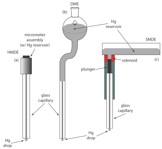
In the dropping mercury electrode, or DME, mercury drops form at the end of the capillary tube as a result of gravity (Figure 11.4.1 b). Unlike the HMDE, the mercury drop of a DME grows continuously—as mercury flows from the reservoir under the influence of gravity—and has a finite lifetime of several seconds. At the end of its lifetime the mercury drop is dislodged, either manually or on its own, and is replaced by a new drop. The static mercury drop electrode, or SMDE, uses a solenoid driven plunger to control the flow of mercury (Figure 11.4.1 c). Activation of the solenoid momentarily lifts the plunger, allowing mercury to flow through the capillary, forming a single, hanging Hg drop. Repeated activation of the solenoid produces a series of Hg drops. In this way the SMDE may be used as either a HMDE or a DME. There is one additional type of mercury electrode: the mercury film electrode. A solid electrode—typically carbon, platinum, or gold—is placed in a solution of Hg2+ and held at a potential where the reduction of Hg2+ to Hg is favorable, depositing a thin film of mercury on the solid electrode’s surface.
Mercury has several advantages as a working electrode. Perhaps its most important advantage is its high overpotential for the reduction of H3O+ to H2, which makes accessible potentials as negative as –1 V versus the SCE in acidic solutions and –2 V versus the SCE in basic solutions (Figure 11.4.2 ). A species such as Zn2+, which is difficult to reduce at other electrodes without simultaneously reducing H3O+, is easy to reduce at a mercury working electrode. Other advantages include the ability of metals to dissolve in mercury—which results in the formation of an amalgam—and the ability to renew the surface of the electrode by extruding a new drop. One limitation to mercury as a working electrode is the ease with which it is oxidized. Depending on the solvent, a mercury electrode can not be used at potentials more positive than approximately –0.3 V to +0.4 V versus the SCE.
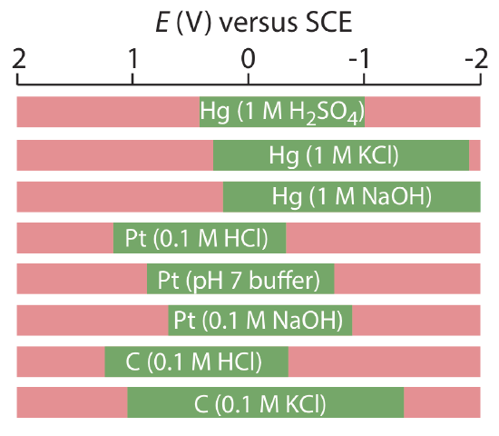
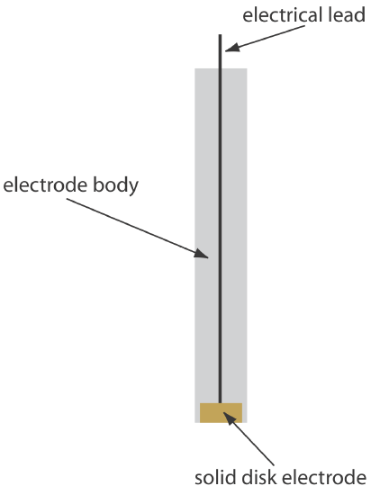
Solid electrodes constructed using platinum, gold, silver, or carbon may be used over a range of potentials, including potentials that are negative and positive with respect to the SCE (Figure 11.4.2 ). For example, the potential window for a Pt electrode extends from approximately +1.2 V to –0.2 V versus the SCE in acidic solutions, and from +0.7 V to –1 V versus the SCE in basic solutions. A solid electrode can replace a mercury electrode for many voltammetric analyses that require negative potentials, and is the electrode of choice at more positive potentials. Except for the carbon paste electrode, a solid electrode is fashioned into a disk and sealed into the end of an inert support with an electrical lead (Figure 11.4.3 ). The carbon paste electrode is made by filling the cavity at the end of the inert support with a paste that consists of carbon particles and a viscous oil. Solid electrodes are not without problems, the most important of which is the ease with which the electrode’s surface is altered by the adsorption of a solution species or by the formation of an oxide layer. For this reason a solid electrode needs frequent reconditioning, either by applying an appropriate potential or by polishing.
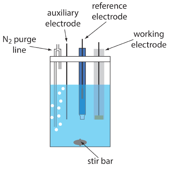
A typical arrangement for a voltammetric electrochemical cell is shown in Figure 11.4.4 . In addition to the working electrode, the reference electrode, and the auxiliary electrode, the cell also includes a N2-purge line for removing dissolved O2, and an optional stir bar. Electrochemical cells are available in a variety of sizes, allowing the analysis of solution volumes ranging from more than 100 mL to as small as 50 μL.
Current In Voltammetry
When we oxidize an analyte at the working electrode, the resulting electrons pass through the potentiostat to the auxiliary electrode, reducing the solvent or some other component of the solution matrix. If we reduce the analyte at the working electrode, the current flows from the auxiliary electrode to the cathode. In either case, the current from the redox reactions at the working electrode and the auxiliary electrodes is called a faradaic current. In this section we consider the factors affecting the magnitude of the faradaic current, as well as the sources of any non-faradaic currents.
Sign Conventions
Because the reaction of interest occurs at the working electrode, we describe the faradaic current using this reaction. A faradaic current due to the analyte’s reduction is a cathodic current, and its sign is positive. An anodic current results from the analyte’s oxidation at the working electrode, and its sign is negative.
Influence of Applied Potential on the Faradaic Current
As an example, let’s consider the faradaic current when we reduce \(\text{Fe(CN)}_6^{3-}\) to \(\text{Fe(CN)}_6^{4-}\) at the working electrode. The relationship between the concentrations of \(\text{Fe(CN)}_6^{3-}\), the concentration of \(\text{Fe(CN)}_6^{4-}\), and the potential is given by the Nernst equation
\[E=+0.356 \text{ V}-0.05916 \log \frac{\left[\mathrm{Fe}(\mathrm{CN})_{6}^{4-}\right]_{x=0}}{\left[\mathrm{Fe}(\mathrm{CN})_{6}^{3-}\right]_{x=0}} \nonumber\]
where +0.356V is the standard-statepotential for the \(\text{Fe(CN)}_6^{3-}\)/\(\text{Fe(CN)}_6^{4-}\) redox couple, and x = 0 indicates that the concentrations of \(\text{Fe(CN)}_6^{3-}\)- and \(\text{Fe(CN)}_6^{4-}\) are those at the surface of the working electrode. We use surface concentrations instead of bulk concentrations because the equilibrium position for the redox reaction
\[\mathrm{Fe}(\mathrm{CN})_{6}^{3-}(a q)+e^{-}\rightleftharpoons\mathrm{Fe}(\mathrm{CN})_{6}^{4-}(a q) \nonumber\]
is established at the electrode’s surface.
Let’s assume we have a solution for which the initial concentration of \(\text{Fe(CN)}_6^{3-}\) is 1.0 mM and that \(\text{Fe(CN)}_6^{4-}\) is absent. Figure 11.4.5 shows the ladder diagram for this solution.
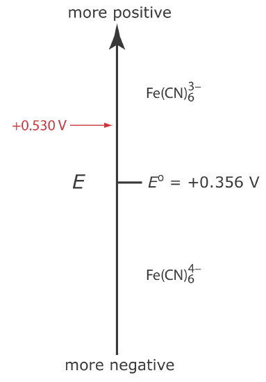
If we apply a potential of +0.530 V to the working electrode, the concentrations of \(\text{Fe(CN)}_6^{3-}\) and \(\text{Fe(CN)}_6^{4-}\) at the surface of the electrode are unaffected, and no faradaic current is observed. If we switch the potential to +0.356 V some of the \(\text{Fe(CN)}_6^{3-}\) at the electrode’s surface is reduced to \(\text{Fe(CN)}_6^{4-}\)until we reach a condition where
\[\left[\mathrm{Fe}(\mathrm{CN})_{6}^{3-}\right]_{x=0}=\left[\mathrm{Fe}(\mathrm{CN})_{6}^{4-}\right]_{x=0}=0.50 \text{ mM} \nonumber\]
This is the first of the five important principles of electrochemistry outlined in Chapter 11.1: the electrode’s potential determines the analyte’s form at the electrode’s surface.
If this is all that happens after we apply the potential, then there would be a brief surge of faradaic current that quickly returns to zero, which is not the most interesting of results. Although the concentrations of \(\text{Fe(CN)}_6^{3-}\) and \(\text{Fe(CN)}_6^{4-}\) at the electrode surface are 0.50 mM, their concentrations in bulk solution remains unchanged.
This is the second of the five important principles of electrochemistry outlined in Chapter 11.1: the analyte’s concentration at the electrode may not be the same as its concentration in bulk solution.
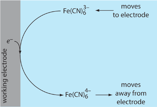
Because of this difference in concentration, there is a concentration gradient between the solution at the electrode’s surface and the bulk solution. This concentration gradient creates a driving force that transports \(\text{Fe(CN)}_6^{4-}\) away from the electrode and that transports \(\text{Fe(CN)}_6^{3-}\) to the electrode (Figure 11.4.6 ). As the \(\text{Fe(CN)}_6^{3-}\) arrives at the electrode it, too, is reduced to \(\text{Fe(CN)}_6^{4-}\). A faradaic current continues to flow until there is no difference between the concentrations of \(\text{Fe(CN)}_6^{3-}\) and \(\text{Fe(CN)}_6^{4-}\) at the electrode and their concentrations in bulk solution.
Although the potential at the working electrode determines if a faradaic current flows, the magnitude of the current is determined by the rate of the resulting oxidation or reduction reaction. Two factors contribute to the rate of the electrochemical reaction: the rate at which the reactants and products are transported to and from the electrode—what we call mass transport—and the rate at which electrons pass between the electrode and the reactants and products in solution.
This is the fourth of the five important principles of electrochemistry outlined in Chapter 11.1: current is a measure of rate.
Influence of Mass Transport on the Faradaic Current
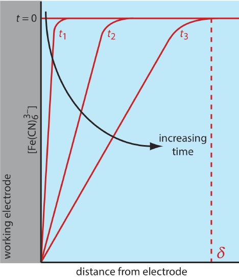
There are three modes of mass transport that affect the rate at which reactants and products move toward or away from the electrode surface: diffusion, migration, and convection. Diffusion occurs whenever the concentration of an ion or a molecule at the surface of the electrode is different from that in bulk solution. If we apply a potential sufficient to completely reduce \(\text{Fe(CN)}_6^{3-}\) at the electrode surface, the result is a concentration gradient similar to that shown in Figure 11.4.7 . The region of solution over which diffusion occurs is the diffusion layer. In the absence of other modes of mass transport, the width of the diffusion layer, \(\delta\), increases with time as the \(\text{Fe(CN)}_6^{3-}\) must diffuse from an increasingly greater distance.
Convection occurs when we mix the solution, which carries reactants toward the electrode and removes products from the electrode. The most common form of convection is stirring the solution with a stir bar; other methods include rotating the electrode and incorporating the electrode into a flow-cell.
The final mode of mass transport is migration, which occurs when a charged particle in solution is attracted to or repelled from an electrode that carries a surface charge. If the electrode carries a positive charge, for example, an anion will move toward the electrode and a cation will move toward the bulk solution. Unlike diffusion and convection, migration affects only the mass transport of charged particles.
The movement of material to and from the electrode surface is a complex function of all three modes of mass transport. In the limit where diffusion is the only significant form of mass transport, the current in a voltammetric cell is equal to
\[i=\frac{n F A D\left(C_{\text {bulk }}-C_{x=0}\right)}{\delta} \label{11.1}\]
where n the number of electrons in the redox reaction, F is Faraday’s constant, A is the area of the electrode, D is the diffusion coefficient for the species reacting at the electrode, Cbulk and Cx = 0 are its concentrations in bulk solution and at the electrode surface, and \(\delta\) is the thickness of the diffusion layer.
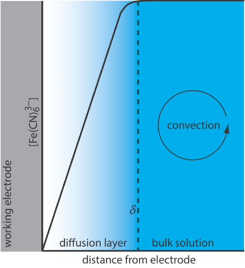
For Equation \ref{11.1} to be valid, convection and migration must not interfere with the formation of a diffusion layer. We can eliminate migration by adding a high concentration of an inert supporting electrolyte. Because ions of similar charge equally are attracted to or repelled from the surface of the electrode, each has an equal probability of undergoing migration. A large excess of an inert electrolyte ensures that few reactants or products experience migration. Although it is easy to eliminate convection by not stirring the solution, there are experimental designs where we cannot avoid convection, either because we must stir the solution or because we are using an electrochemical flow cell. Fortunately, as shown in Figure 11.4.8 , the dynamics of a fluid moving past an electrode results in a small diffusion layer—typically 1–10 μm in thickness—in which the rate of mass transport by convection drops to zero.
Effect of Electron Transfer Kinetics on the Faradaic Current
The rate of mass transport is one factor that influences the current in voltammetry. The ease with which electrons move between the electrode and the species that reacts at the electrode also affects the current. When electron transfer kinetics are fast, the redox reaction is at equilibrium. Under these conditions the redox reaction is electrochemically reversible and the Nernst equation applies. If the electron transfer kinetics are sufficiently slow, the concentration of reactants and products at the electrode surface—and thus the magnitude of the faradaic current—are not what is predicted by the Nernst equation. In this case the system is electrochemically irreversible.
Charging Currents
In addition to the faradaic current from a redox reaction, the current in an electrochemical cell includes other, nonfaradaic sources. Suppose the charge on an electrode is zero and we suddenly change its potential so that the electrode’s surface acquires a positive charge. Cations near the electrode’s surface will respond to this positive charge by migrating away from the electrode; anions, on the other hand, will migrate toward the electrode. This migration of ions occurs until the electrode’s positive surface charge and the negative charge of the solution near the electrode are equal. Because the movement of ions and the movement of electrons are indistinguishable, the result is a small, short-lived nonfaradaic current that we call the charging current. Every time we change the electrode’s potential, a transient charging current flows.
The migration of ions in response to the electrode’s surface charge leads to the formation of a structured electrode-solution interface that we call the electrical double layer, or EDL. When we change an electrode’s potential, the charging current is the result of a restructuring of the EDL. The exact structure of the electrical double layer is not important in the context of this text, but you can consult this chapter’s additional resources for additional information.
Residual Current
Even in the absence of analyte, a small, measurable current flows through an electrochemical cell. This residual current has two components: a faradaic current due to the oxidation or reduction of trace impurities and a nonfaradaic charging current. Methods for discriminating between the analyte’s faradaic current and the residual current are discussed later in this chapter.
Shape of Voltammograms
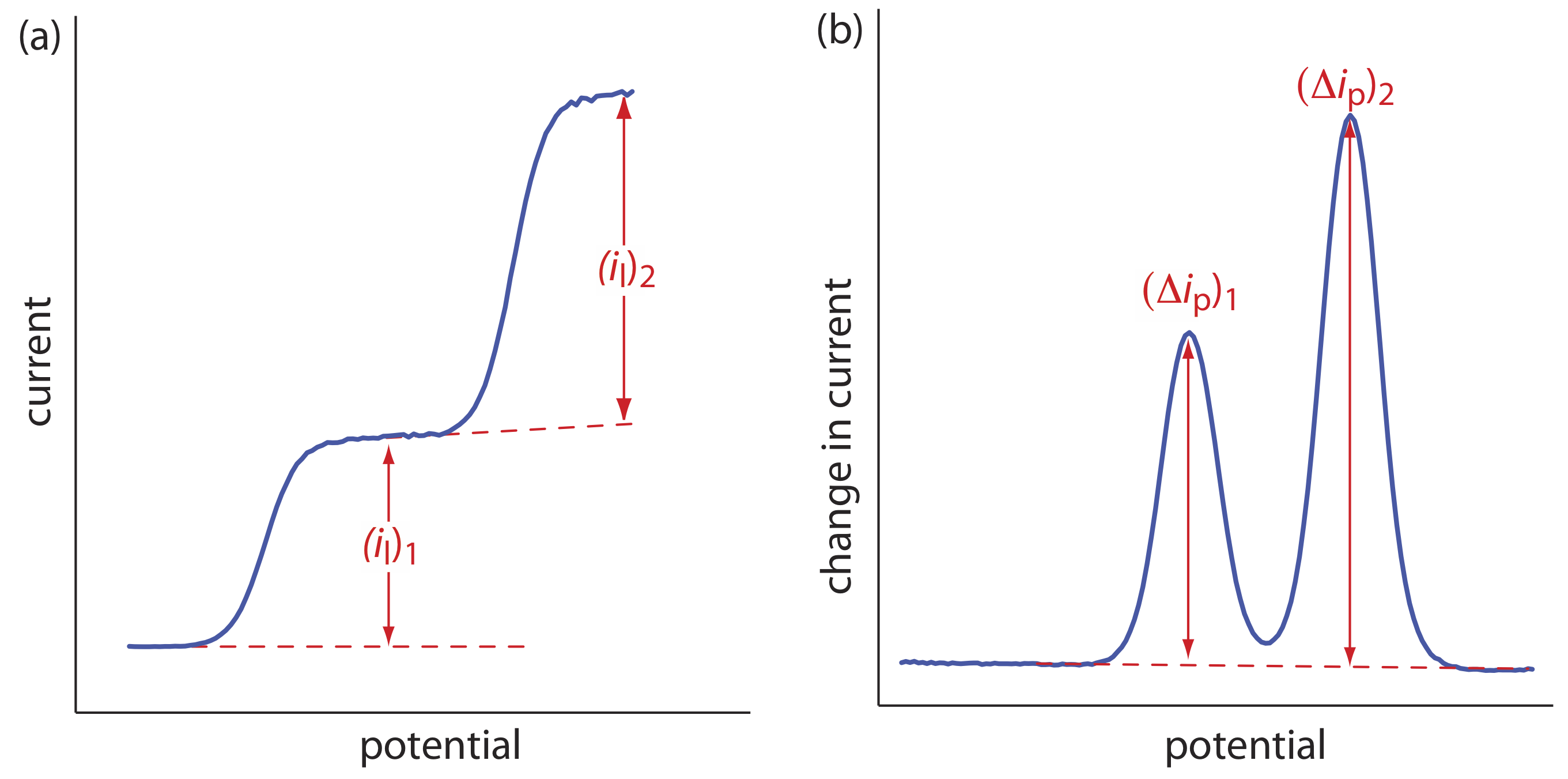
The shape of a voltammogram is determined by several experimental factors, the most important of which are how we measure the current and whether convection is included as a means of mass transport. As shown in Figure 11.4.9 , despite an abundance of different voltammetric techniques, several of which are discussed in this chapter, there are only three common shapes for voltammograms.
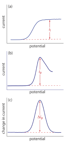
For the voltammogram in Figure 11.4.9 a, the current increases from a background residual current to a limiting current, il. Because the faradaic current is inversely proportional to \(\delta\) (Equation \ref{11.1}), a limiting current occurs only if the thickness of the diffusion layer remains constant because we are stirring the solution (see Figure 11.4.8 ). In the absence of convection the diffusion layer increases with time (see Figure 11.4.7 ). As shown in Figure 11.4.9 b, the resulting voltammogram has a peak current instead of a limiting current.
For the voltammograms in Figure 11.4.9 a and Figure 11.4.9 b, we measure the current as a function of the applied potential. We also can monitor the change in current, \(\Delta i\), following a change in potential. The resulting voltammogram, shown in Figure 11.4.9 c, also has a peak current.
Quantitative and Qualitative Aspects of Voltammetry
Earlier we described a voltammogram as the electrochemical equivalent of a spectrum in spectroscopy. In this section we consider how we can extract quantitative and qualitative information from a voltammogram. For simplicity we will limit our treatment to voltammograms similar to Figure 11.4.9 a.
Determining Concentration
Let’s assume that the redox reaction at the working electrode is
\[O+n e^{-} \rightleftharpoons R \label{11.2}\]
where O is the analyte’s oxidized form and R is its reduced form. Let’s also assume that only O initially is present in bulk solution and that we are stirring the solution. When we apply a potential that results in the reduction of O to R, the current depends on the rate at which O diffuses through the fixed diffusion layer shown in Figure 11.4.7 . Using Equation \ref{11.1}, the current, i, is
\[i=K_{O}\left([O]_{\text {bulk }}-[O]_{x=0}\right) \label{11.3}\]
where KO is a constant equal to \(n F A D_O / \delta\). When we reach the limiting current, il, the concentration of O at the electrode surface is zero and Equation \ref{11.3} simplifies to
\[i_{l}=K_{O}[O]_{\mathrm{bulk}} \label{11.4}\]
Equation \ref{11.4} shows us that the limiting current is a linear function of the concentration of O in bulk solution. To determine the value of KO we can use any of the standardization methods covered in Chapter 5. Equations similar to Equation \ref{11.4} can be developed for the other two types of voltammograms shown in Figure 11.4.9 .
Determining the Standard-State Potential
To extract the standard-state potential from a voltammogram, we need to rewrite the Nernst equation for reaction \ref{11.2}
\[E=E_{O / R}^{\circ}-\frac{0.05916}{n} \log \frac{[R]_{x=0}}{[O]_{x=0}} \label{11.5}\]
in terms of current instead of the concentrations of O and R. We will do this in several steps. First, we substitute Equation \ref{11.4} into Equation \ref{11.3} and rearrange to give
\[[O]_{x=0}=\frac{i_{l}-i}{K_{O}} \label{11.6}\]
Next, we derive a similar equation for [R]x = 0, by noting that
\[i=K_{R}\left([R]_{x=0}-[R]_{\mathrm{bulk}}\right) \nonumber\]
Because the concentration of [R]bulk is zero—remember our assumption that the initial solution contains only O—we can simplify this equation
\[i=K_{R}[R]_{x=0} \nonumber\]
and solve for [R]x = 0.
\[[R]_{x=0}=\frac{i}{K_{R}} \label{11.7}\]
Now we are ready to finish our derivation. Substituting Equation \ref{11.7} and Equation \ref{11.6} into Equation \ref{11.5} and rearranging leaves us with
\[E=E_{O / R}^{\circ}-\frac{0.05916}{n} \log \frac{K_{O}}{K_{R}}-\frac{0.05916}{n} \log \frac{i}{i_{l} - i} \label{11.8}\]
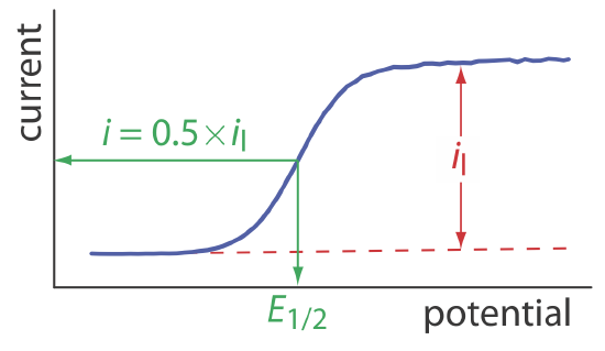
When the current, i, is half of the limiting current, il,
\[i=0.5 \times i_{l} \nonumber\]
we can simplify Equation \ref{11.8} to
\[E_{1 / 2}=E_{O / R}^{\circ}-\frac{0.05916}{n} \log \frac{K_{O}}{K_{R}} \label{11.9}\]
where E1/2 is the half-wave potential (Figure 11.4.10 ). If KO is approximately equal to KR, which often is the case, then the half-wave potential is equal to the standard-state potential. Note that Equation \ref{11.9} is valid only if the redox reaction is electrochemically reversible.
Voltammetric Techniques
In voltammetry there are three important experimental parameters under our control: how we change the potential applied to the working electrode, when we choose to measure the current, and whether we choose to stir the solution. Not surprisingly, there are many different voltammetric techniques. In this section we consider several important examples.
Polarography
The first important voltammetric technique to be developed—polarography—uses the dropping mercury electrode shown in Figure 11.4.1 b as the working electrode. As shown in Figure 11.4.11 , the current is measured while applying a linear potential ramp.
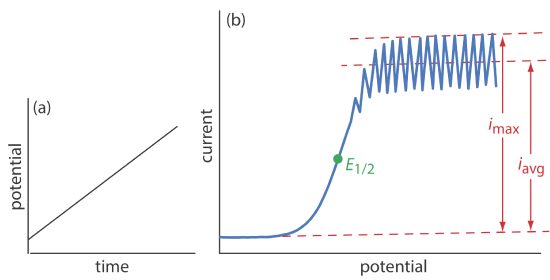
Although polarography takes place in an unstirred solution, we obtain a limiting current instead of a peak current. When a Hg drop separates from the glass capillary and falls to the bottom of the electrochemical cell, it mixes the solution. Each new Hg drop, therefore, grows into a solution whose composition is identical to the bulk solution. The oscillations in the current are a result of the Hg drop’s growth, which leads to a time-dependent change in the area of the working electrode. The limiting current—which also is called the diffusion current—is measured using either the maximum current, imax, or from the average current, iavg. The relationship between the analyte’s concentration, CA, and the limiting current is given by the Ilkovic equations
\[i_{\max }=706 n D^{1 / 2} m^{2 / 3} t^{1 / 6} C_{A}=K_{\max } C_{A} \nonumber\]
\[i_{avg}=607 n D^{1 / 2} m^{2 / 3} t^{1 / 6} C_{A}=K_{\mathrm{avg}} C_{A} \nonumber\]
where n is the number of electrons in the redox reaction, D is the analyte’s diffusion coefficient, m is the flow rate of Hg, t is the drop’s lifetime and Kmax and Kavg are constants. The half-wave potential, E1/2, provides qualitative information about the redox reaction.
Normal polarography has been replaced by various forms of pulse polarography, several examples of which are shown in Figure 11.4.12 [Osteryoung, J. J. Chem. Educ. 1983, 60, 296–298]. Normal pulse polarography (Figure 11.4.12 a), for example, uses a series of potential pulses characterized by a cycle of time \(\tau\), a pulse-time of tp, a pulse potential of \(\Delta E_\text{p}\), and a scan rate of \(\Delta E / \Delta t\). Typical experimental conditions for normal pulse polarography are \(\tau \approx 1 \text{ s}\), tp ≈ 50 ms, and \(\Delta E / \Delta t \approx 2 \text{ mV/s}\). The initial value of \(\Delta E_\text{p} \approx 2 \text{ mV}\), and it increases by ≈ 2 mV with each pulse. The current is sampled at the end of each potential pulse for approximately 17 ms before returning the potential to its initial value. The shape of the resulting voltammogram is similar to Figure 11.4.11 , but without the current oscillations. Because we apply the potential for only a small portion of the drop’s lifetime, there is less time for the analyte to undergo oxidation or reduction and a smaller diffusion layer. As a result, the faradaic current in normal pulse polarography is greater than in the polarography, resulting in better sensitivity and smaller detection limits.
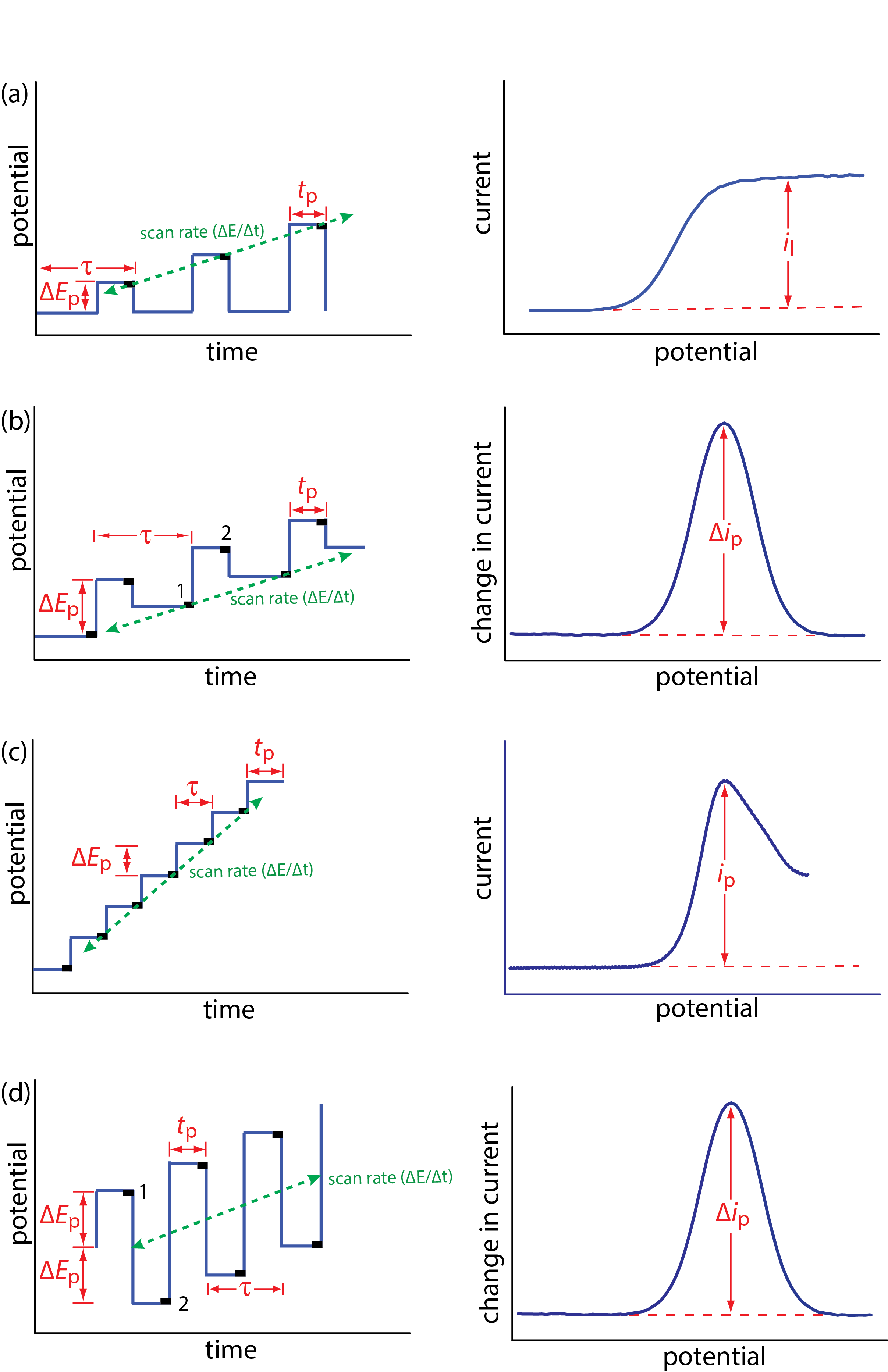
In differential pulse polarography (Figure 11.4.12 b) the current is measured twice per cycle: for approximately 17 ms before applying the pulse and for approximately 17 ms at the end of the cycle. The difference in the two currents gives rise to the peak-shaped voltammogram. Typical experimental conditions for differential pulse polarography are \(\tau \approx 1 \text{ s}\), tp ≈ 50 ms, \(\Delta E_\text{p}\) ≈ 50 mV, and \(\Delta E / \Delta t\) ≈ 2 mV/s.
The voltammogram for differential pulse polarography is approximately the first derivative of the voltammogram for normal pulse polarography. To see why this is the case, note that the change in current over a fixed change in potential, \(\Delta i / \Delta E\), approximates the slope of the voltammogram for normal pulse polarography. You may recall that the first derivative of a function returns the slope of the function at each point. The first derivative of a sigmoidal function is a peak-shaped function.
Other forms of pulse polarography include staircase polarography (Figure 11.4.12 c) and square-wave polarography (Figure 11.4.12 d). One advantage of square-wave polarography is that we can make \(\tau\) very small—perhaps as small as 5 ms, compared to 1 s for other forms of pulse polarography—which significantly decreases analysis time. For example, suppose we need to scan a potential range of 400 mV. If we use normal pulse polarography with a \(\Delta E / \Delta t\) of 2 mV/cycle and a \(\tau\) of 1 s/cycle, then we need 200 s to complete the scan. If we use square-wave polarography with a \(\Delta E / \Delta t\) of 2 mV/cycle and a \(\tau\) of 5 ms/cycle, we can complete the scan in 1 s. At this rate, we can acquire a complete voltammogram using a single drop of Hg!
Polarography is used extensively for the analysis of metal ions and inorganic anions, such as \(\text{IO}_3^-\) and \(\text{NO}_3^-\). We also can use polarography to study organic compounds with easily reducible or oxidizable functional groups, such as carbonyls, carboxylic acids, and carbon-carbon double bonds.
Hydrodynamic Voltammetry
In polarography we obtain a limiting current because each drop of mercury mixes the solution as it falls to the bottom of the electrochemical cell. If we replace the DME with a solid electrode (see Figure 11.4.3 ), we can still obtain a limiting current if we mechanically stir the solution during the analysis, using either a stir bar or by rotating the electrode. We call this approach hydrodynamic voltammetry.
Hydrodynamic voltammetry uses the same potential profiles as in polarography, such as a linear scan (Figure 11.4.11 ) or a differential pulse (Figure 11.4.12 b). The resulting voltammograms are identical to those for polarography, except for the lack of current oscillations from the growth of the mercury drops. Because hydrodynamic voltammetry is not limited to Hg electrodes, it is useful for analytes that undergo oxidation or reduction at more positive potentials.
Stripping Voltammetry
Another important voltammetric technique is stripping voltammetry, which consists of three related techniques: anodic stripping voltammetry, cathodic stripping voltammetry, and adsorptive stripping voltammetry. Because anodic stripping voltammetry is the more widely used of these techniques, we will consider it in greatest detail.
Anodic stripping voltammetry consists of two steps (Figure 11.4.13 ). The first step is a controlled potential electrolysis in which we hold the working electrode—usually a hanging mercury drop or a mercury film electrode—at a cathodic potential sufficient to deposit the metal ion on the electrode. For example, when analyzing Cu2+ the deposition reaction is
\[\mathrm{Cu}^{2+}+2 e^{-} \rightleftharpoons \mathrm{Cu}(\mathrm{Hg}) \nonumber\]
where Cu(Hg) indicates that the copper is amalgamated with the mercury. This step serves as a means of concentrating the analyte by transferring it from the larger volume of the solution to the smaller volume of the electrode. During most of the electrolysis we stir the solution to increase the rate of deposition. Near the end of the deposition time we stop the stirring—eliminating convection as a mode of mass transport—and allow the solution to become quiescent. Typical deposition times of 1–30 min are common, with analytes at lower concentrations requiring longer times.
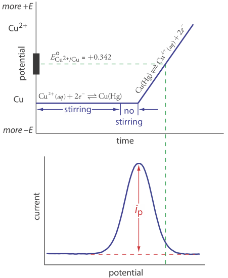
In the second step, we scan the potential anodically—that is, toward a more positive potential. When the working electrode’s potential is sufficiently positive, the analyte is stripped from the electrode, returning to solution in its oxidized form.
\[\mathrm{Cu}(\mathrm{Hg})\rightleftharpoons \text{ Cu}^{2+}+2 e^{-} \nonumber\]
Monitoring the current during the stripping step gives a peak-shaped voltammogram, as shown in Figure 11.4.13 . The peak current is proportional to the analyte’s concentration in the solution. Because we are concentrating the analyte in the electrode, detection limits are much smaller than other electrochemical techniques. An improvement of three orders of magnitude—the equivalent of parts per billion instead of parts per million—is routine.
Anodic stripping voltammetry is very sensitive to experimental conditions, which we must carefully control to obtain results that are accurate and precise. Key variables include the area of the mercury film or the size of the hanging Hg drop, the deposition time, the rest time, the rate of stirring, and the scan rate during the stripping step. Anodic stripping voltammetry is particularly useful for metals that form amalgams with mercury, several examples of which are listed in Table 11.4.1 .
The experimental design for cathodic stripping voltammetry is similar to anodic stripping voltammetry with two exceptions. First, the deposition step involves the oxidation of the Hg electrode to \(\text{Hg}_2^{2+}\), which then reacts with the analyte to form an insoluble film at the surface of the electrode. For example, when Cl– is the analyte the deposition step is
\[2 \mathrm{Hg}(l)+2 \mathrm{Cl}^{-}(a q) \rightleftharpoons \text{ Hg}_{2} \mathrm{Cl}_{2}(s)+2 e^{-} \nonumber\]
Second, stripping is accomplished by scanning cathodically toward a more negative potential, reducing \(\text{Hg}_2^{2+}\) back to Hg and returning the analyte to solution.
\[\mathrm{Hg}_{2} \mathrm{Cl}_{2}(s)+2 e^{-}\rightleftharpoons 2 \mathrm{Hg}( l)+2 \mathrm{Cl}^{-}(a q) \nonumber\]
Table 11.4.1 lists several analytes analyzed successfully by cathodic stripping voltammetry.
In adsorptive stripping voltammetry, the deposition step occurs without electrolysis. Instead, the analyte adsorbs to the electrode’s surface. During deposition we maintain the electrode at a potential that enhances adsorption. For example, we can adsorb a neutral molecule on a Hg drop if we apply a potential of –0.4 V versus the SCE, a potential where the surface charge of mercury is approximately zero. When deposition is complete, we scan the potential in an anodic or a cathodic direction, depending on whether we are oxidizing or reducing the analyte. Examples of compounds that have been analyzed by absorptive stripping voltammetry also are listed in Table 11.4.1 .
Cyclic Voltammetry
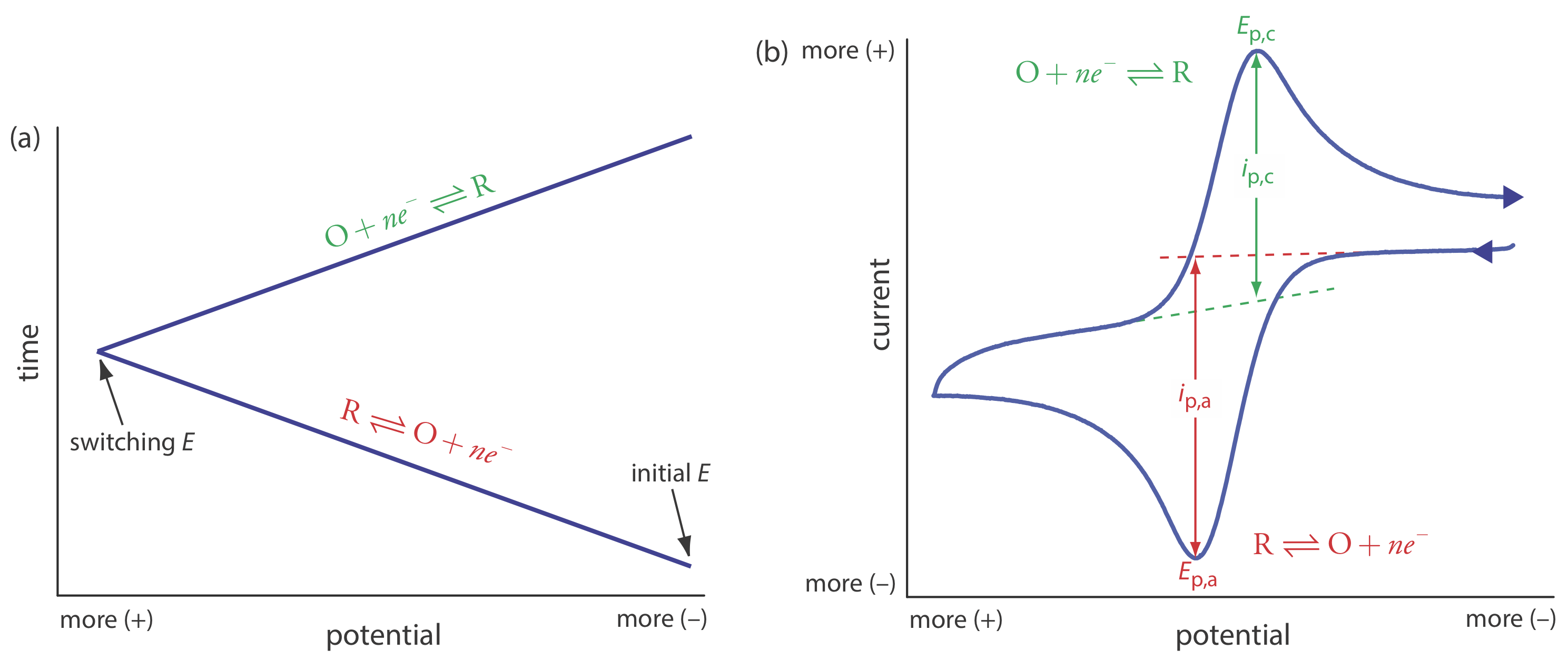
In the voltammetric techniques consider to this point we scan the potential in one direction, either to more positive potentials or to more negative potentials. In cyclic voltammetry we complete a scan in both directions. Figure 11.4.14 a shows a typical potential-excitation signal. In this example, we first scan the potential to more positive values, resulting in the following oxidation reaction for the species R.
\[R \rightleftharpoons O+n e^{-} \nonumber\]
When the potential reaches a predetermined switching potential, we reverse the direction of the scan toward more negative potentials. Because we generated the species O on the forward scan, during the reverse scan it reduces back to R.
\[O+n e^{-} \rightleftharpoons R \nonumber\]
Cyclic voltammetry is carried out in an unstirred solution, which, as shown in Figure 11.4.14 b, results in peak currents instead of limiting currents. The voltammogram has separate peaks for the oxidation reaction and for the reduction reaction, each characterized by a peak potential and a peak current.
The peak current in cyclic voltammetry is given by the Randles-Sevcik equation
\[i_{p}=\left(2.69 \times 10^{5}\right) n^{3 / 2} A D^{1 / 2} \nu^{1 / 2} C_{A} \nonumber\]
where n is the number of electrons in the redox reaction, A is the area of the working electrode, D is the diffusion coefficient for the electroactive species, \(\nu\) is the scan rate, and CA is the concentration of the electroactive species at the electrode. For a well-behaved system, the anodic and the cathodic peak currents are equal, and the ratio ip,a/ip,c is 1.00. The half-wave potential, E1/2, is midway between the anodic and cathodic peak potentials.
\[E_{1 / 2}=\frac{E_{p, a}+E_{p, c}}{2} \nonumber\]
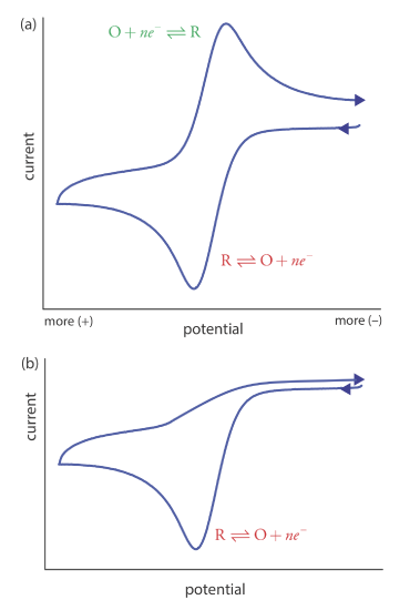
Scanning the potential in both directions provides an opportunity to explore the electrochemical behavior of species generated at the electrode. This is a distinct advantage of cyclic voltammetry over other voltammetric techniques. Figure 11.4.15 shows the cyclic voltammogram for the same redox couple at both a faster and a slower scan rate. At the faster scan rate, 11.4.15 a, we see two peaks. At the slower scan rate in Figure 11.4.15 b, however, the peak on the reverse scan disappears. One explanation for this is that the products from the reduction of R on the forward scan have sufficient time to participate in a chemical reaction whose products are not electroactive.
Amperometry
The final voltammetric technique we will consider is amperometry, in which we apply a constant potential to the working electrode and measure current as a function of time. Because we do not vary the potential, amperometry does not result in a voltammogram.
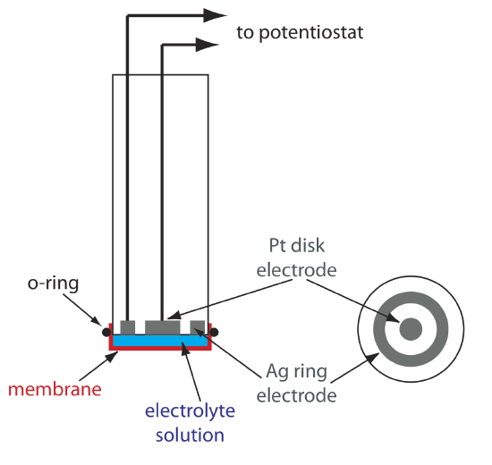
One important application of amperometry is in the construction of chemical sensors. One of the first amperometric sensors was developed in 1956 by L. C. Clark to measure dissolved O2 in blood. Figure 11.4.16 shows the sensor’s design, which is similar to a potentiometric membrane electrode. A thin, gas-permeable membrane is stretched across the end of the sensor and is separated from the working electrode and the counter electrode by a thin solution of KCl. The working electrode is a Pt disk cathode, and a Ag ring anode serves as the counter electrode. Although several gases can diffuse across the membrane, including O2, N2, and CO2, only oxygen undergoes reduction at the cathode
\[\mathrm{O}_{2}(g)+4 \mathrm{H}_{3} \mathrm{O}^{+}(a q)+4 e^{-}\rightleftharpoons 6 \mathrm{H}_{2} \mathrm{O}(l) \nonumber\]
with its concentration at the electrode’s surface quickly reaching zero. The concentration of O2 at the membrane’s inner surface is fixed by its diffusion through the membrane, which creates a diffusion profile similar to that in Figure 11.4.8 . The result is a steady-state current that is proportional to the concentration of dissolved oxygen. Because the electrode consumes oxygen,the sample is stirred to prevent the depletion of O2 at the membrane’s outer surface.
The oxidation of the Ag anode is the other half-reaction.
\[\mathrm{Ag}(s)+\text{ Cl}^{-}(a q)\rightleftharpoons \mathrm{AgCl}(s)+e^{-} \nonumber\]
Another example of an amperometric sensor is a glucose sensor. In this sensor the single membrane in Figure 11.4.16 is replaced with three membranes. The outermost membrane of polycarbonate is permeable to glucose and O2. The second membrane contains an immobilized preparation of glucose oxidase that catalyzes the oxidation of glucose to gluconolactone and hydrogen peroxide.
\[\beta-\mathrm{D}-\text {glucose }(a q)+\text{ O}_{2}(a q)+\mathrm{H}_{2} \mathrm{O}(l)\rightleftharpoons \text {gluconolactone }(a q)+\text{ H}_{2} \mathrm{O}_{2}(a q) \nonumber\]
The hydrogen peroxide diffuses through the innermost membrane of cellulose acetate where it undergoes oxidation at a Pt anode.
\[\mathrm{H}_{2} \mathrm{O}_{2}(a q)+2 \mathrm{OH}^{-}(a q) \rightleftharpoons \text{ O}_{2}(a q)+2 \mathrm{H}_{2} \mathrm{O}(l)+2 e^{-} \nonumber\]
Figure 11.4.17 summarizes the reactions that take place in this amperometric sensor. FAD is the oxidized form of flavin adenine nucleotide—the active site of the enzyme glucose oxidase—and FADH2 is the active site’s reduced form. Note that O2 serves a mediator, carrying electrons to the electrode.
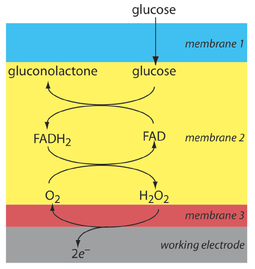
By changing the enzyme and mediator, it is easy to extend to the amperometric sensor in Figure 11.4.17 to the analysis of other analytes. For example, a CO2 sensor has been developed using an amperometric O2 sensor with a two-layer membrane, one of which contains an immobilized preparation of autotrophic bacteria [Karube, I.; Nomura, Y.; Arikawa, Y. Trends in Anal. Chem. 1995, 14, 295–299]. As CO2 diffuses through the membranes it is converted to O2 by the bacteria, increasing the concentration of O2 at the Pt cathode.
Quantitative Applications
Voltammetry has been used for the quantitative analysis of a wide variety of samples, including environmental samples, clinical samples, pharmaceutical formulations, steels, gasoline, and oil.
Selecting the Voltammetric Technique
The choice of which voltammetric technique to use depends on the sample’s characteristics, including the analyte’s expected concentration and the sample’s location. For example, amperometry is ideally suited for detecting analytes in flow systems, including the in vivo analysis of a patient’s blood or as a selective sensor for the rapid analysis of a single analyte. The portability of amperometric sensors, which are similar to potentiometric sensors, also make them ideal for field studies. Although cyclic voltammetry is used to determine an analyte’s concentration, other methods described in this chapter are better suited for quantitative work.
Pulse polarography and stripping voltammetry frequently are interchangeable. The choice of which technique to use often depends on the analyte’s concentration and the desired accuracy and precision. Detection limits for normal pulse polarography generally are on the order of 10–6 M to 10–7 M, and those for differential pulse polarography, staircase, and square wave polarography are between 10–7 M and 10–9 M. Because we concentrate the analyte in stripping voltammetry, the detection limit for many analytes is as little as 10–10 M to 10–12 M. On the other hand, the current in stripping voltammetry is much more sensitive than pulse polarography to changes in experimental conditions, which may lead to poorer precision and accuracy. We also can use pulse polarography to analyze a wider range of inorganic and organic analytes because there is no need to first deposit the analyte at the electrode surface.
Stripping voltammetry also suffers from occasional interferences when two metals, such as Cu and Zn, combine to form an intermetallic compound in the mercury amalgam. The deposition potential for Zn . is sufficiently negative that any Cu2+ in the sample also deposits into the mercury drop or film, leading to the formation of intermetallic compounds such as CuZn and CuZn2. During the stripping step, zinc in the intermetallic compounds strips at potentials near that of copper, decreasing the current for zinc at its usual potential and increasing the apparent current for copper. It is possible to overcome this problem by adding an element that forms a stronger intermetallic compound with the interfering metal. Thus, adding Ga3+ minimizes the interference of Cu when analyzing for Zn by forming an intermetallic compound of Cu and Ga.
Correcting the Residual Current
In any quantitative analysis we must correct the analyte’s signal for signals that arise from other sources. The total current, itot, in voltammetry consists of two parts: the current from the analyte’s oxidation or reduction, iA, and a background or residual current, ir.
\[i_{t o t}=i_{A}+i_{r} \nonumber\]
The residual current, in turn, has two sources. One source is a faradaic current from the oxidation or reduction of trace interferents in the sample, iint. The other source is the charging current, ich, that accompanies a change in the working electrode’s potential.
\[i_{r}=i_{\mathrm{int}}+i_{c h} \nonumber\]
We can minimize the faradaic current due to impurities by carefully preparing the sample. For example, one important impurity is dissolved O2, which undergoes a two-step reduction: first to H2O2 at a potential of –0.1 V versus the SCE, and then to H2O at a potential of –0.9 V versus the SCE. Removing dissolved O2 by bubbling an inert gas such as N2 through the sample eliminates this interference. After removing the dissolved O2, maintaining a blanket of N2 over the top of the solution prevents O2 from reentering the solution.
The cell in Figure 11.4.4 shows a typical N2 purge line.
There are two methods to compensate for the residual current. One method is to measure the total current at potentials where the analyte’s faradaic current is zero and extrapolate it to other potentials. This is the method shown in Figure 11.4.9 . One advantage of extrapolating is that we do not need to acquire additional data. An important disadvantage is that an extrapolation assumes that any change in the residual current with potential is predictable, which may not be the case. A second, and more rigorous approach, is to obtain a voltammogram for an appropriate blank. The blank’s residual current is then subtracted from the sample’s total current.
Analysis for Single Components
The analysis of a sample with a single analyte is straightforward using any of the standardization methods discussed in Chapter 5.
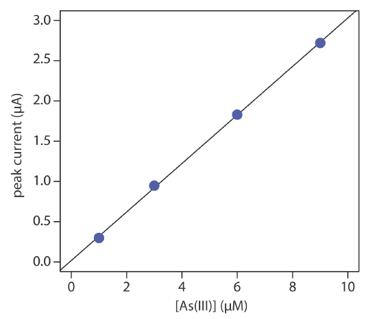
The concentration of As(III) in water is determined by differential pulse polarography in 1 M HCl. The initial potential is set to –0.1 V versus the SCE and is scanned toward more negative potentials at a rate of 5 mV/s. Reduction of As(III) to As(0) occurs at a potential of approximately –0.44 V versus the SCE. The peak currents for a set of standard solutions, corrected for the residual current, are shown in the following table.
| [As(III)] (µM) | ip (µM) |
|---|---|
| 1.00 | 0.298 |
| 3.00 | 0.947 |
| 6.00 | 1.83 |
| 9.00 | 2.72 |
What is the concentration of As(III) in a sample of water if its peak current is 1.37 μA?
Solution
Linear regression gives the calibration curve shown in Figure 11.4.18 , with an equation of
\[i_{p}=0.0176+3.01 \times[\mathrm{As}(\mathrm{III})] \nonumber\]
Substituting the sample’s peak current into the regression equation gives the concentration of As(III) as 4.49 μM.
The concentration of copper in a sample of sea water is determined by anodic stripping voltammetry using the method of standard additions. The analysis of a 50.0-mL sample gives a peak current of 0.886 μA. After adding a 5.00-μL spike of 10.0 mg/L Cu2+, the peak current increases to 2.52 μA. Calculate the μg/L copper in the sample of sea water.
- Answer
-
For anodic stripping voltammetry, the peak current, ip, is a linear function of the analyte’s concentration
\[i_{p}=K \times C_{\mathrm{Cu}} \nonumber\]
where K is a constant that accounts for experimental parameters such as the electrode’s area, the diffusion coefficient for Cu2+, the deposition time, and the rate of stirring. For the analysis of the sample before the standard addition we know that the current is
\[i_{p}=0.886 \ \mu \mathrm{A}=K \times C_{\mathrm{Cu}} \nonumber\]
and after the standard addition the current is
\[i_{p}=2.52 \ \mu \mathrm{A}=K\left\{C_{\mathrm{Cu}} \times \frac{50.00 \ \mathrm{mL}}{50.005 \ \mathrm{mL}}+\frac{10.00 \mathrm{mg} \mathrm{Cu}}{\mathrm{L}} \times \frac{0.005 \ \mathrm{mL}}{50.005 \ \mathrm{mL}}\right\} \nonumber\]
where 50.005 mL is the total volume after we add the 5.00 μL spike. Solving each equation for K and combining leaves us with the following equation.
\[\frac{0.886 \ \mu \mathrm{A}}{C_{\mathrm{Cu}}}=K=\frac{2.52 \ \mu \mathrm{A}}{C_{\mathrm{Cu}} \times \frac{50.00 \ \mathrm{mL}}{50.005 \ \mathrm{mL}}+\frac{10.00 \ \mathrm{mg} \text{ Cu}}{\mathrm{L}} \times \frac{0.005 \ \mathrm{mL}}{50.005 \ \mathrm{mL}}} \nonumber\]
Solving this equation for CCu gives its value as \(5.42 \times 10^{-4}\) mg Cu2+/L, or 0.542 μg Cu2+/L.
Multicomponent Analysis
Voltammetry is a particularly attractive technique for the analysis of samples that contain two or more analytes. Provided that the analytes behave independently, the voltammogram of a multicomponent mixture is a summation of each analyte’s individual voltammograms. As shown in Figure 11.4.19 , if the separation between the half-wave potentials or between the peak potentials is sufficient, we can determine the presence of each analyte as if it is the only analyte in the sample. The minimum separation between the half-wave potentials or peak potentials for two analytes depends on several factors, including the type of electrode and the potential-excitation signal. For normal polarography the separation is at least ±0.2–0.3 V, and differential pulse voltammetry requires a minimum separation of ±0.04–0.05 V.
If the voltammograms for two analytes are not sufficiently separated, a simultaneous analysis may be possible. An example of this approach is outlined the following example.
The differential pulse polarographic analysis of a mixture of indium and cadmium in 0.1 M HCl is complicated by the overlap of their respective voltammograms [Lanza P. J. Chem. Educ. 1990, 67, 704–705]. The peak potential for indium is at –0.557 V and that for cadmium is at –0.597 V. When a 0.800-ppm indium standard is analyzed, \(\Delta i_p\) (in arbitrary units) is 200.5 at –0.557 V and 87.5 at –0.597 V relative to a saturated Ag/AgCl reference electorde. A standard solution of 0.793 ppm cadmium has a \(\Delta i_p\) of 58.5 at –0.557 V and 128.5 at –0.597 V. What is the concentration of indium and cadmium in a sample if \(\Delta i_p\) is 167.0 at a potential of –0.557 V and 99.5 at a potential of –0.597V.
Solution
The change in current, \(\Delta i_p\), in differential pulse polarography is a linear function of the analyte’s concentration
\[\Delta i_{p}=k_{A} C_{A} \nonumber\]
where kA is a constant that depends on the analyte and the applied potential, and CA is the analyte’s concentration. To determine the concentrations of indium and cadmium in the sample we must first find the value of kA for each analyte at each potential. For simplicity we will identify the potential of –0.557 V as E1, and that for –0.597 V as E2. The values of kA are
\[\begin{aligned} k_{\mathrm{In}, E_{1}} &=\frac{200.5}{0.800 \ \mathrm{ppm}}=250.6 \ \mathrm{ppm}^{-1} \\ k_{\mathrm{In}, E_{2}} &=\frac{87.5}{0.800 \ \mathrm{ppm}}=109.4 \ \mathrm{ppm}^{-1} \\ k_{\mathrm{Cd} E_{1}} &=\frac{58.5}{0.793 \ \mathrm{ppm}}=73.8 \ \mathrm{ppm}^{-1} \\ k_{\mathrm{Cd} E_{2}} &=\frac{128.5}{0.793 \ \mathrm{ppm}}=162.0 \ \mathrm{ppm}^{-1} \end{aligned} \nonumber\]
Next, we write simultaneous equations for the current at the two potentials.
\[\begin{array}{l}{\Delta i_{E_{1}}=167.0=250.6 \ \mathrm{ppm}^{-1} \times C_{\mathrm{In}}+73.8 \ \mathrm{ppm}^{-1} \times C_{\mathrm{Cd}}} \\ {\triangle i_{E_{2}}=99.5=109.4 \ \mathrm{ppm}^{-1} \times C_{\mathrm{In}}+162.0 \ \mathrm{ppm}^{-1} \times C_{\mathrm{Cd}}}\end{array} \nonumber\]
Solving the simultaneous equations, which is left as an exercise, gives the concentration of indium as 0.606 ppm and the concentration of cadmium as 0.205 ppm.
Environmental Samples
Voltammetry is one of several important analytical techniques for the analysis of trace metals in environmental samples, including groundwater, lakes, rivers and streams, seawater, rain, and snow. Detection limits at the parts-per-billion level are routine for many trace metals using differential pulse polarography, with anodic stripping voltammetry providing parts-per-trillion detection limits for some trace metals.
One interesting environmental application of anodic stripping voltammetry is the determination of a trace metal’s chemical form within a water sample. Speciation is important because a trace metal’s bioavailability, toxicity, and ease of transport through the environment often depends on its chemical form. For example, a trace metal that is strongly bound to colloidal particles generally is not toxic because it is not available to aquatic lifeforms. Unfortunately, anodic stripping voltammetry can not distinguish a trace metal’s exact chemical form because closely related species, such as Pb2+ and PbCl+, produce a single stripping peak. Instead, trace metals are divided into “operationally defined” categories that have environmental significance.
Operationally defined means that an analyte is divided into categories by the specific methods used to isolate it from the sample. There are many examples of operational definitions in the environmental literature. The distribution of trace metals in soils and sediments, for example, often is defined in terms of the reagents used to extract them; thus, you might find an operational definition for Zn2+ in a lake sediment as that extracted using 1.0 M sodium acetate, or that extracted using 1.0 M HCl.
Although there are many speciation schemes in the environmental literature, we will consider one proposed by Batley and Florence [see (a) Batley, G. E.; Florence, T. M. Anal. Lett. 1976, 9, 379–388; (b) Batley, G. E.; Florence, T. M. Talanta 1977, 24, 151–158; (c) Batley, G. E.; Florence, T. M. Anal. Chem. 1980, 52, 1962–1963; (d) Florence, T. M., Batley, G. E.; CRC Crit. Rev. Anal. Chem. 1980, 9, 219–296]. This scheme, which is outlined in Table 11.4.2 , combines anodic stripping voltammetry with ion-exchange and UV irradiation, dividing soluble trace metals into seven groups. In the first step, anodic stripping voltammetry in a pH 4.8 acetic acid buffer differentiates between labile metals and nonlabile metals. Only labile metals—those present as hydrated ions, weakly bound complexes, or weakly adsorbed on colloidal surfaces—deposit at the electrode and give rise to a signal. Total metal concentration are determined by ASV after digesting the sample in 2 M HNO3 for 5 min, which converts all metals into an ASV-labile form.
A Chelex-100 ion-exchange resin further differentiates between strongly bound metals—usually metals bound to inorganic and organic solids, but also those tightly bound to chelating ligands—and more loosely bound metals. Finally, UV radiation differentiates between metals bound to organic phases and inorganic phases. The analysis of seawater samples, for example, suggests that cadmium, copper, and lead are present primarily as labile organic complexes or as labile adsorbates on organic colloids (Group II in Table 11.4.2 ).
Differential pulse polarography and stripping voltammetry are used to determine trace metals in airborne particulates, incinerator fly ash, rocks, minerals, and sediments. The trace metals, of course, are first brought into solution using a digestion or an extraction.
Amperometric sensors also are used to analyze environmental samples. For example, the dissolved O2 sensor described earlier is used to determine the level of dissolved oxygen and the biochemical oxygen demand, or BOD, of waters and wastewaters. The latter test—which is a measure of the amount of oxygen required by aquatic bacteria as they decompose organic matter—is important when evaluating the efficiency of a wastewater treatment plant and for monitoring organic pollution in natural waters. A high BOD suggests that the water has a high concentration of organic matter. Decomposition of this organic matter may seriously deplete the level of dissolved oxygen in the water, adversely affecting aquatic life. Other amperometric sensors are available to monitor anionic surfactants in water, and CO2, H2SO4, and NH3 in atmospheric gases.
Clinical Samples
Differential pulse polarography and stripping voltammetry are used to determine the concentration of trace metals in a variety of clinical samples, including blood, urine, and tissue. The determination of lead in blood is of considerable interest due to concerns about lead poisoning. Because the concentration of lead in blood is so small, anodic stripping voltammetry frequently is the more appropriate technique. The analysis is complicated, however, by the presence of proteins that may adsorb to the mercury electrode, inhibiting either the deposition or stripping of lead. In addition, proteins may prevent the electrodeposition of lead through the formation of stable, nonlabile complexes. Digesting and ashing the blood sample mini- mizes this problem. Differential pulse polarography is useful for the routine quantitative analysis of drugs in biological fluids, at concentrations of less than 10–6 M [Brooks, M. A. “Application of Electrochemistry to Pharmaceutical Analysis,” Chapter 21 in Kissinger, P. T.; Heinemann, W. R., eds. Laboratory Techniques in Electroanalytical Chemistry, Marcel Dekker, Inc.: New York, 1984, pp 539–568.]. Amperometric sensors using enzyme catalysts also have many clinical uses, several examples of which are shown in Table 11.4.3 .
Miscellaneous Samples
In addition to environmental samples and clinical samples, differential pulse polarography and stripping voltammetry are used for the analysis of trace metals in other sample, including food, steels and other alloys, gasoline, gunpowder residues, and pharmaceuticals. Voltammetry is an important technique for the quantitative analysis of organics, particularly in the pharmaceutical industry where it is used to determine the concentration of drugs and vitamins in formulations. For example, voltammetric methods are available for the quantitative analysis of vitamin A, niacinamide, and riboflavin. When the compound of interest is not electroactive, it often can be derivatized to an electroactive form. One example is the differential pulse polarographic determination of sulfanilamide, which is converted into an electroactive azo dye by coupling with sulfamic acid and 1-napthol.
Representative Method 11.4.1: Determination of Chloropromazine in a Pharmaceutical Product
The best way to appreciate the theoretical and the practical details discussed in this section is to carefully examine a typical analytical method. Although each method is unique, the following description of the determination of chloropromazine in a pharmaceutical product provides an instructive example of a typical procedure. The description here is based on a method from Pungor, E. A Practical Guide to Instrumental Analysis, CRC Press: Boca Raton, FL, 1995, pp. 34–37.
Description of Method
Chlorpromazine, also is known by its trade name Thorazine, is an antipsychotic drug used in the treatment of schizophrenia. The amount of chlorpromazine in a pharmaceutical product is determined voltammetrically at a graphite working electrode in a unstirred solution, with calibration by the method of standard additions.
Procedure
Add 10.00 mL of an electrolyte solution consisting of 0.01 M HCl and 0.1 M KCl to the electrochemical cell. Place a graphite working electrode, a Pt auxiliary electrode, and a SCE reference electrode in the cell, and record the voltammogram from 0.2 V to 2.0 V at a scan rate of 50 mV/s. Weigh out an appropriate amount of the pharmaceutical product and dissolve it in a small amount of the electrolyte. Transfer the solution to a 100-mL volumetric flask and dilute to volume with the electrolyte. Filter a small amount of the diluted solution and transfer 1.00 mL of the filtrate to the voltammetric cell. Mix the contents of the voltammetric cell and allow the solution to sit for 10 s before recording the voltammogram. Return the potential to 0.2 V, add 1.00 mL of a chlorpromazine standard and record the voltammogram. Report the %w/w chlorpromazine in the formulation.
Questions
1. Is chlorpromazine undergoing oxidation or reduction at the graphite working electrode?
Because we are scanning toward more positive potentials, we are oxidizing chlorpromazine.
2. Why does this procedure use a graphite electrode instead of a Hg electrode?
As shown in Figure 11.4.2 , the potential window for a Hg electrode extends from approximately –0.3 V to between –1V and –2 V, de- pending on the pH. Because we are scanning the potential from 0.2 V to 2.0 V, we cannot use a Hg electrode.
3. Many voltammetric procedures require that we first remove dissolved O2 by bubbling N2 through the solution. Why is this not necessary for this analysis?
Dissolved O2 is a problem when we scan toward more negative potentials, because its reduction may produce a significant cathodic current. In this procedure we are scanning toward more positive potentials and generating anodic currents; thus, dissolved O2 is not an interferent and does not need to be removed.
4. What is the purpose of recording a voltammogram in the absence of chlorpromazine?
This voltammogram serves as a blank, which provides a measurement of the residual current due to the electrolyte. Because the potential window for a graphite working electrode (see Figure 11.4.2 ) does not extend to 2.0 V, there is a measurable anodic residual current due to the solvent’s oxidation. Having measured this residual current, we can subtract it from the total current in the presence of chlorpromazine.
5. Based on the description of this procedure, what is the shape of the resulting voltammogram. You may wish to review the three common shapes shown in Figure 11.4.9 .
Because the solution is unstirred, the voltammogram will have a peak current similar to that shown in Figure 11.4.9 b.
Characterization Applications
In the previous section we learned how to use voltammetry to determine an analyte’s concentration in a variety of different samples. We also can use voltammetry to characterize an analyte’s properties, including verifying its electrochemical reversibility, determining the number of electrons transferred during its oxidation or reduction, and determining its equilibrium constant in a coupled chemical reaction.
Electrochemical Reversibility and Determination of n
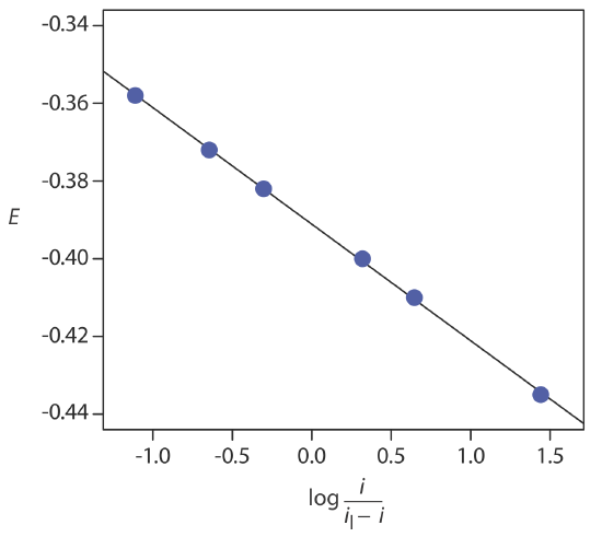
Earlier in this chapter we derived a relationship between E1/2 and the standard-state potential for a redox couple (Equation \ref{11.9}), noting that a redox reaction must be electrochemically reversible. How can we tell if a redox reaction is reversible by looking at its voltammogram? For a reversible redox reaction Equation \ref{11.8}, which we repeat here, describes the relationship between potential and current for a voltammetric experiment with a limiting current.
\[E=E_{O / R}^{\circ}-\frac{0.05916}{n} \log \frac{K_{O}}{K_{R}}-\frac{0.05916}{n} \log \frac{i}{i_{l} - i} \nonumber\]
If a reaction is electrochemically reversible, a plot of E versus log(i/il – i) is a straight line with a slope of –0.05916/n. In addition, the slope should yield an integer value for n.
The following data were obtained from a linear scan hydrodynamic voltammogram of a reversible reduction reaction.
| E (V vs. SCE) | current (μA) |
|---|---|
| –0.358 | 0.37 |
| –0.372 | 0.95 |
| –0.382 | 1.71 |
| –0.400 | 3.48 |
| –0.410 | 4.20 |
| –0.435 | 4.97 |
The limiting current is 5.15 μA. Show that the reduction reaction is reversible, and determine values for n and for E1/2.
Solution
Figure 11.4.20 shows a plot of E versus log(i/il–i). Because the result is a straight-line, we know the reaction is electrochemically reversible under the conditions of the experiment. A linear regression analysis gives the equation for the straight line as
\[E=-0.391 \mathrm{V}-0.0300 \log \frac{i}{i_{l}-i} \nonumber\]
From Equation \ref{11.8}, the slope is equivalent to –0.05916/n; solving for n gives a value of 1.97, or 2 electrons. From Equation \ref{11.8} and Equation \ref{11.9}, we know that E1/2 is the y-intercept for a plot of E versus log(i/il – i); thus, E1/2 for the data in this example is –0.391 V versus the SCE.
We also can use cyclic voltammetry to evaluate electrochemical reversibility by looking at the difference between the peak potentials for the anodic and the cathodic scans. For an electrochemically reversible reaction, the following equation holds true.
\[\Delta E_{p}=E_{p, a}-E_{p, c}=\frac{0.05916 \ \mathrm{V}}{n} \nonumber\]
As an example, for a two-electron reduction we expect a \(\Delta E_p\) of approximately 29.6 mV. For an electrochemically irreversible reaction the value of \(\Delta E_p\) is larger than expected.
Determining Equilibrium Constants for Coupled Chemical Reactions
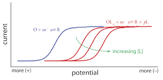
Another important application of voltammetry is determining the equilibrium constant for a solution reaction that is coupled to a redox reaction. The presence of the solution reaction affects the ease of electron transfer in the redox reaction, shifting E1/2 to a more negative or to a more positive potential. Consider, for example, the reduction of O to R
\[O+n e^{-} \rightleftharpoons R \nonumber\]
the voltammogram for which is shown in Figure 11.4.21 . If we introduce a ligand, L, that forms a strong complex with O, then we also must consider the reaction
\[O+p L\rightleftharpoons O L_{p} \nonumber\]
In the presence of the ligand, the overall redox reaction is
\[O L_{p}+n e^{-} \rightleftharpoons R+p L \nonumber\]
Because of its stability, the reduction of the OLp complex is less favorable than the reduction of O. As shown in Figure 11.4.21 , the resulting voltammogram shifts to a potential that is more negative than that for O. Furthermore, the shift in the voltammogram increases as we increase the ligand’s concentration.
We can use this shift in the value of E1/2 to determine both the stoichiometry and the formation constant for a metal-ligand complex. To derive a relationship between the relevant variables we begin with two equations: the Nernst equation for the reduction of O
\[E=E_{O / R}^{\circ}-\frac{0.05916}{n} \log \frac{[R]_{x=0}}{[O]_{x=0}} \label{11.10}\]
and the stability constant, \(\beta_p\) for the metal-ligand complex at the electrode surface.
\[\beta_{p} = \frac{\left[O L_p\right]_{x = 0}}{[O]_{x = 0}[L]_{x = 0}^p} \label{11.11}\]
In the absence of ligand the half-wave potential occurs when [R]x = 0 and [O]x = 0 are equal; thus, from the Nernst equation we have
\[\left(E_{1 / 2}\right)_{n c}=E_{O / R}^{\circ} \label{11.12}\]
where the subscript “nc” signifies that the complex is not present.
When ligand is present we must account for its effect on the concentration of O. Solving Equation \ref{11.1} for [O]x = 0 and substituting into the Equation \ref{11.10} gives
\[E=E_{O/R}^{\circ}-\frac{0.05916}{n} \log \frac{[R]_{x=0}[L]_{x=0}^{p} \beta_{p}}{\left[O L_{p}\right]_{x=0}} \label{11.13}\]
If the formation constant is sufficiently large, such that essentially all O is present as the complex OLp, then [R]x = 0 and [OLp]x = 0 are equal at the half-wave potential, and Equation \ref{11.13} simplifies to
\[\left(E_{1 / 2}\right)_{c} = E_{O/R}^{\circ} - \frac{0.05916}{n} \log{} [L]_{x=0}^{p} \beta_{p} \label{11.14}\]
where the subscript “c” indicates that the complex is present. Defining \(\Delta E_{1/2}\) as
\[\triangle E_{1 / 2}=\left(E_{1 / 2}\right)_{c}-\left(E_{1 / 2}\right)_{n c} \label{11.15}\]
and substituting Equation \ref{11.12} and Equation \ref{11.14} and expanding the log term leaves us with the following equation.
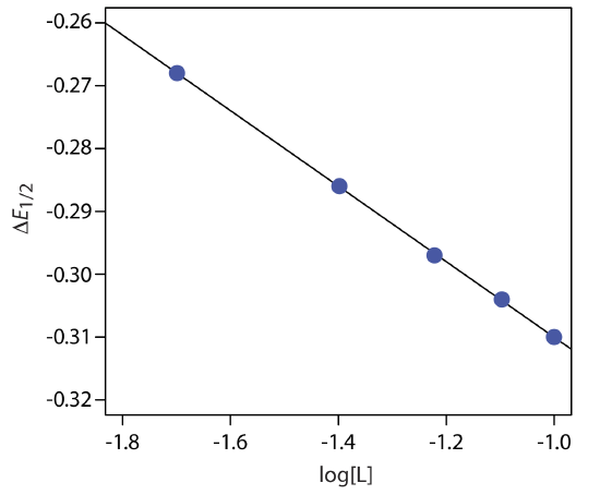
\[\Delta E_{1 / 2}=-\frac{0.05916}{n} \log \beta_{p}-\frac{0.05916 p}{n} \log {[L]} \label{11.16}\]
A plot of \(\Delta E_{1/2}\) versus log[L] is a straight-line, with a slope that is a function of the metal-ligand complex’s stoichiometric coefficient, p, and a y-intercept that is a function of its formation constant \(\beta_p\).
A voltammogram for the two-electron reduction (n = 2) of a metal, M, has a half-wave potential of –0.226 V versus the SCE. In the presence of an excess of ligand, L, the following half-wave potentials are recorded.
| [L] (M) | (E1/2)c (V vs. SCE) |
|---|---|
| 0.020 | –0.494 |
| 0.040 | –0.512 |
| 0.060 | –0.523 |
| 0.080 | –0.530 |
| 0.100 | –0.536 |
Determine the stoichiometry of the metal-ligand complex and its formation constant.
Solution
We begin by calculating values of \(\Delta E_{1/2}\) using Equation \ref{11.15}, obtaining the values in the following table.
| [L] (M) | \(\Delta E_{1/2}\) (V vs. SCE) |
|---|---|
| 0.020 | –0.268 |
| 0.040 | –0.286 |
| 0.060 | –0.297 |
| 0.080 | –0.304 |
| 0.100 | –0.310 |
Figure 11.4.22 shows the resulting plot of \(\Delta E_{1/2}\) as a function of log[L]. A linear regression analysis gives the equation for the straight line as
\[\triangle E_{1 / 2}=-0.370 \mathrm{V}-0.0601 \log {[L]} \nonumber\]
From Equation \ref{11.16} we know that the slope is equal to –0.05916p/n. Using the slope and n = 2, we solve for p obtaining a value of 2.03 ≈ 2. The complex’s stoichiometry, therefore, is ML2. We also know, from Equation \ref{11.16}, that the y-intercept is equivalent to –(0.05916/n)log\(\beta_p\). Solving for \(\beta_2\) gives a formation constant of \(3.2 \times 10^{12}\).
The voltammogram for 0.50 mM Cd2+ has an E1/2 of –0.565 V versus an SCE. After making the solution 0.115 M in ethylenediamine, E1/2 is –0.845 V, and E1/2 is –0.873 V when the solution is 0.231 M in ethylenediamine. Determine the stoichiometry of the Cd2+–ethylenediamine complex and its formation constant. The data in this problem comes from Morinaga, K. “Polarographic Studies of Metal Complexes. V. Ethylenediamine Complexes of Cadmium, Nickel, and Zinc,” Bull. Chem. Soc. Japan 1956, 29, 793–799.
- Answer
-
For simplicity, we will use en as a shorthand notation for ethylenediamine. From the three half-wave potentials we have a \(\Delta E_{1/2}\) of –0.280 V for 0.115 M en and a \(\Delta E_{1/2}\) of –0.308 V for 0.231 M en. Using Equation \ref{11.16} we write the following two equations.
\[\begin{array}{l}{-0.280=-\frac{0.05916}{2} \log \beta_{p}-\frac{0.05916 p}{2} \log (0.115)} \\ {-0.308=-\frac{0.05916}{2} \log \beta_{p}-\frac{0.05916 p}{2} \log (0.231)}\end{array} \nonumber\]
To solve for the value of p, we first subtract the second equation from the first equation
\[0.028=-\frac{0.05916 p}{2} \log (0.115)-\left\{-\frac{0.05916 p}{2} \log (0.231)\right\} \nonumber\]
which eliminates the term with \(\beta_p\). Next we solve this equation for p
\[0.028=\left(2.778 \times 10^{-2}\right) \times p-\left(1.882 \times 10^{-2}\right) \times p =\left(8.96 \times 10^{-3}\right) \times p \nonumber\]
obtaining a value of 3.1, or p ≈ 3. Thus, the complex is Cd(en)3. To find the formation complex, \(\beta_3\), we return to Equation \ref{11.16}, using our value for p. Using the data for an en concentration of 0.115 M
\[\begin{aligned}-0.280=-& \frac{0.05916}{2} \log \beta_{3}-\frac{0.05916 \times 3}{2} \log (0.115) \\ &-0.363=-\frac{0.05916}{2} \log \beta_{3} \end{aligned} \nonumber\]
gives a value for \(\beta_3\) of \(1.92 \times 10^{12}\). Using the data for an en concentration of 0.231 M gives a value of \(2.10 \times 10^{12}\).
As suggested by Figure 11.4.15 , cyclic voltammetry is one of the most powerful electrochemical techniques for exploring the mechanism of coupled electrochemical and chemical reactions. The treatment of this aspect of cyclic voltammetry is beyond the level of this text, although you can consult this chapter’s additional resources for additional information.
Evaluation
Scale of Operation
Detection levels at the parts-per-million level are routine. For some analytes and for some voltammetric techniques, lower detection limits are possible. Detection limits at the parts-per-billion and the part-per-trillion level are possible with stripping voltammetry. Although most analyses are carried out in conventional electrochemical cells using macro samples, the availability of microelectrodes with diameters as small as 2 μm, allows for the analysis of samples with volumes under 50 μL. For example, the concentration of glucose in 200-μm pond snail neurons was monitored successfully using an amperometric glucose electrode with a 2 mm tip [Abe, T.; Lauw, L. L.; Ewing, A. G. J. Am. Chem. Soc. 1991, 113, 7421–7423].
Accuracy
The accuracy of a voltammetric analysis usually is limited by our ability to correct for residual currents, particularly those due to charging. For an analyte at the parts-per-million level, an accuracy of ±1–3% is routine. Accuracy decreases for samples with significantly smaller concentrations of analyte.
Precision
Precision generally is limited by the uncertainty in measuring the limiting current or the peak current. Under most conditions, a precision of ±1–3% is reasonable. One exception is the analysis of ultratrace analytes in complex matrices by stripping voltammetry, in which the precision may be as poor as ±25%.
Sensitivity
In many voltammetric experiments, we can improve the sensitivity by adjusting the experimental conditions. For example, in stripping voltammetry we can improve sensitivity by increasing the deposition time, by increasing the rate of the linear potential scan, or by using a differential-pulse technique. One reason that potential pulse techniques are popular is that they provide an improvement in current relative to a linear potential scan.
Selectivity
Selectivity in voltammetry is determined by the difference between half-wave potentials or peak potentials, with a minimum difference of ±0.2–0.3 V for a linear potential scan and ±0.04–0.05 V for differential pulse voltammetry. We often can improve selectivity by adjusting solution conditions. The addition of a complexing ligand, for example, can substantially shift the potential where a species is oxidized or reduced to a potential where it no longer interferes with the determination of an analyte. Other solution parameters, such as pH, also can be used to improve selectivity.
Time, Cost, and Equipment
Commercial instrumentation for voltammetry ranges from <$1000 for simple instruments to >$20,000 for a more sophisticated instrument. In general, less expensive instrumentation is limited to linear potential scans. More expensive instruments provide for more complex potential-excitation signals using potential pulses. Except for stripping voltammetry, which needs a long deposition time, voltammetric analyses are relatively rapid.