
6.5: Collision Theory, Activation Energy, and the Arrhenius Equation
- Page ID
- 499148

\( \newcommand{\vecs}[1]{\overset { \scriptstyle \rightharpoonup} {\mathbf{#1}} } \)
\( \newcommand{\vecd}[1]{\overset{-\!-\!\rightharpoonup}{\vphantom{a}\smash {#1}}} \)
\( \newcommand{\dsum}{\displaystyle\sum\limits} \)
\( \newcommand{\dint}{\displaystyle\int\limits} \)
\( \newcommand{\dlim}{\displaystyle\lim\limits} \)
\( \newcommand{\id}{\mathrm{id}}\) \( \newcommand{\Span}{\mathrm{span}}\)
( \newcommand{\kernel}{\mathrm{null}\,}\) \( \newcommand{\range}{\mathrm{range}\,}\)
\( \newcommand{\RealPart}{\mathrm{Re}}\) \( \newcommand{\ImaginaryPart}{\mathrm{Im}}\)
\( \newcommand{\Argument}{\mathrm{Arg}}\) \( \newcommand{\norm}[1]{\| #1 \|}\)
\( \newcommand{\inner}[2]{\langle #1, #2 \rangle}\)
\( \newcommand{\Span}{\mathrm{span}}\)
\( \newcommand{\id}{\mathrm{id}}\)
\( \newcommand{\Span}{\mathrm{span}}\)
\( \newcommand{\kernel}{\mathrm{null}\,}\)
\( \newcommand{\range}{\mathrm{range}\,}\)
\( \newcommand{\RealPart}{\mathrm{Re}}\)
\( \newcommand{\ImaginaryPart}{\mathrm{Im}}\)
\( \newcommand{\Argument}{\mathrm{Arg}}\)
\( \newcommand{\norm}[1]{\| #1 \|}\)
\( \newcommand{\inner}[2]{\langle #1, #2 \rangle}\)
\( \newcommand{\Span}{\mathrm{span}}\) \( \newcommand{\AA}{\unicode[.8,0]{x212B}}\)
\( \newcommand{\vectorA}[1]{\vec{#1}} % arrow\)
\( \newcommand{\vectorAt}[1]{\vec{\text{#1}}} % arrow\)
\( \newcommand{\vectorB}[1]{\overset { \scriptstyle \rightharpoonup} {\mathbf{#1}} } \)
\( \newcommand{\vectorC}[1]{\textbf{#1}} \)
\( \newcommand{\vectorD}[1]{\overrightarrow{#1}} \)
\( \newcommand{\vectorDt}[1]{\overrightarrow{\text{#1}}} \)
\( \newcommand{\vectE}[1]{\overset{-\!-\!\rightharpoonup}{\vphantom{a}\smash{\mathbf {#1}}}} \)
\( \newcommand{\vecs}[1]{\overset { \scriptstyle \rightharpoonup} {\mathbf{#1}} } \)
\(\newcommand{\longvect}{\overrightarrow}\)
\( \newcommand{\vecd}[1]{\overset{-\!-\!\rightharpoonup}{\vphantom{a}\smash {#1}}} \)
\(\newcommand{\avec}{\mathbf a}\) \(\newcommand{\bvec}{\mathbf b}\) \(\newcommand{\cvec}{\mathbf c}\) \(\newcommand{\dvec}{\mathbf d}\) \(\newcommand{\dtil}{\widetilde{\mathbf d}}\) \(\newcommand{\evec}{\mathbf e}\) \(\newcommand{\fvec}{\mathbf f}\) \(\newcommand{\nvec}{\mathbf n}\) \(\newcommand{\pvec}{\mathbf p}\) \(\newcommand{\qvec}{\mathbf q}\) \(\newcommand{\svec}{\mathbf s}\) \(\newcommand{\tvec}{\mathbf t}\) \(\newcommand{\uvec}{\mathbf u}\) \(\newcommand{\vvec}{\mathbf v}\) \(\newcommand{\wvec}{\mathbf w}\) \(\newcommand{\xvec}{\mathbf x}\) \(\newcommand{\yvec}{\mathbf y}\) \(\newcommand{\zvec}{\mathbf z}\) \(\newcommand{\rvec}{\mathbf r}\) \(\newcommand{\mvec}{\mathbf m}\) \(\newcommand{\zerovec}{\mathbf 0}\) \(\newcommand{\onevec}{\mathbf 1}\) \(\newcommand{\real}{\mathbb R}\) \(\newcommand{\twovec}[2]{\left[\begin{array}{r}#1 \\ #2 \end{array}\right]}\) \(\newcommand{\ctwovec}[2]{\left[\begin{array}{c}#1 \\ #2 \end{array}\right]}\) \(\newcommand{\threevec}[3]{\left[\begin{array}{r}#1 \\ #2 \\ #3 \end{array}\right]}\) \(\newcommand{\cthreevec}[3]{\left[\begin{array}{c}#1 \\ #2 \\ #3 \end{array}\right]}\) \(\newcommand{\fourvec}[4]{\left[\begin{array}{r}#1 \\ #2 \\ #3 \\ #4 \end{array}\right]}\) \(\newcommand{\cfourvec}[4]{\left[\begin{array}{c}#1 \\ #2 \\ #3 \\ #4 \end{array}\right]}\) \(\newcommand{\fivevec}[5]{\left[\begin{array}{r}#1 \\ #2 \\ #3 \\ #4 \\ #5 \\ \end{array}\right]}\) \(\newcommand{\cfivevec}[5]{\left[\begin{array}{c}#1 \\ #2 \\ #3 \\ #4 \\ #5 \\ \end{array}\right]}\) \(\newcommand{\mattwo}[4]{\left[\begin{array}{rr}#1 \amp #2 \\ #3 \amp #4 \\ \end{array}\right]}\) \(\newcommand{\laspan}[1]{\text{Span}\{#1\}}\) \(\newcommand{\bcal}{\cal B}\) \(\newcommand{\ccal}{\cal C}\) \(\newcommand{\scal}{\cal S}\) \(\newcommand{\wcal}{\cal W}\) \(\newcommand{\ecal}{\cal E}\) \(\newcommand{\coords}[2]{\left\{#1\right\}_{#2}}\) \(\newcommand{\gray}[1]{\color{gray}{#1}}\) \(\newcommand{\lgray}[1]{\color{lightgray}{#1}}\) \(\newcommand{\rank}{\operatorname{rank}}\) \(\newcommand{\row}{\text{Row}}\) \(\newcommand{\col}{\text{Col}}\) \(\renewcommand{\row}{\text{Row}}\) \(\newcommand{\nul}{\text{Nul}}\) \(\newcommand{\var}{\text{Var}}\) \(\newcommand{\corr}{\text{corr}}\) \(\newcommand{\len}[1]{\left|#1\right|}\) \(\newcommand{\bbar}{\overline{\bvec}}\) \(\newcommand{\bhat}{\widehat{\bvec}}\) \(\newcommand{\bperp}{\bvec^\perp}\) \(\newcommand{\xhat}{\widehat{\xvec}}\) \(\newcommand{\vhat}{\widehat{\vvec}}\) \(\newcommand{\uhat}{\widehat{\uvec}}\) \(\newcommand{\what}{\widehat{\wvec}}\) \(\newcommand{\Sighat}{\widehat{\Sigma}}\) \(\newcommand{\lt}{<}\) \(\newcommand{\gt}{>}\) \(\newcommand{\amp}{&}\) \(\definecolor{fillinmathshade}{gray}{0.9}\)- Define the concepts of activation energy and transition state
- Explain the dependence of rate on concentration and temperature using collision theory
- Relate the temperature, activation energy, and rate constant through the Arrhenius equation
For a chemical reaction to occur, reactant atoms, molecules, or ions must collide. Since atoms must be close together to form chemical bonds, the frequency and nature of these collisions determine reaction rates. Collision theory explains how molecular collisions lead to reactions and why some reactions occur faster than others.
- The rate of a reaction is proportional to the rate of reactant collisions: \[\mathrm{reaction\: rate ∝ \dfrac{\#\,collisions}{time}} \nonumber \]
- Molecules must collide with the correct orientation so that the atoms involved in bond formation make contact.
- Collisions must have enough energy to break existing bonds and form new ones. This minimum energy requirement is called the activation energy (Ea).
Consider the reaction of carbon monoxide, a pollutant produced from the combustion of fuels, with oxygen:
\[\ce{2CO}(g)+\ce{O2}(g)⟶\ce{2CO2}(g) \nonumber \]
This reaction is crucial for reducing carbon monoxide emissions from vehicles. The first step in the gas-phase reaction between carbon monoxide and oxygen is a collision between the two molecules:
\[\ce{CO}(g)+\ce{O2}(g)⟶\ce{CO2}(g)+\ce{O}(g) \nonumber \]
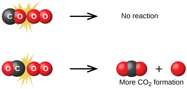
However, not all collisions between CO and O2 molecules lead to products. Molecules can collide in many different orientations, but only certain alignments allow the reaction to occur. Figure \(\PageIndex{1}\) shows just two possibilities:
- If the oxygen end of the CO molecule collides with O2, the reaction is unlikely because the carbon and oxygen atoms needed to form \(\ce{CO2}\) are not properly aligned.
- If the carbon end of the CO molecule collides with O2, the reaction is more likely to proceed, forming carbon dioxide (O=C=O).
If the oxygen end of the CO molecule collides with O2 (first case), the reaction is unlikely to occur because the carbon and oxygen atoms needed to form CO2 line up. The second case is more likely to result in the formation of carbon dioxide, which has a central carbon atom bonded to two oxygen atoms (\(\ce{O=C=O}\)). This example demonstrates how molecular orientation is a factor in determining whether a collision is successful.
Not all collisions with the correct orientation result in the formation of products. Collisions must also occur with sufficient energy for the reaction to take place. This minimum required energy is called the activation energy (Ea). Reactant molecules must collide with enough energy to reach a transition state, a high-energy intermediate in which bonds are partially broken and formed. We will explore activation energies and transition states further in the next section.
Collision theory also explains how reaction rates depend on concentration. When the concentration of a reactant increases, the number of molecular collisions per unit time also increases. More collisions lead to a faster reaction rate, provided that the colliding molecules have enough energy to overcome the activation barrier.
Activation Energy
The activation energy, Ea, is the minimum energy required for a reaction to occur. Figure \(\PageIndex{2}\) shows the energy profile for a general reaction:
\[A+B⟶C+D \nonumber \]
The activation energy for the forward reaction is the energy difference between the reactants and the transition state, a high-energy intermediate.
As reactants approach each other, their kinetic energy is converted into potential energy as they reach the transition state. If the reactants do not have sufficient energy to reach the transition state products will not form, reactants \(A\) and \(B\) will reform and potential energy will be transformed back into kinetic energy.
If \(A\) and \(B\) collide with sufficient energy to reach the transition state it can transform back into reactants \(A\) and \(B\) or into products \(C\) and \(D\). The transition state is the highest energy species between reactants and products and so it represents the energy barrier required to transform reactants into products but forward progress is not guaranteed and the observed rate of reaction includes the probability of the transition state transforming back to reactants or forward towards products. If the transition state proceeds towards products, the potential energy of the transition state is converted to chemical energy of the bonds formed and broken as well as the resulting kinetic energy of the products.
The chemical energy stored in the bonds of the products is not always the same as that of the reactants and \(ΔH\) represents the energy difference between the potential energies of the reactants (\(A\) and \(B\)) and the products (\(C\) and \(D\)). If the products have a lower potential energy than the reactants this energy will be transferred to the products as kinetic energy, which will be transferred to surrounding molecules, increasing their overall average kinetic energy or temperature. This is an example of an exothermic reaction, and is what is represented in Figure \(\PageIndex{2}\). Conversely, if the products have a higher potential energy than the reactants they will receive less kinetic energy, which will decrease the overall kinetic energy of the surrounding molecules, decreasing the temperature. This is an endothermic reaction.
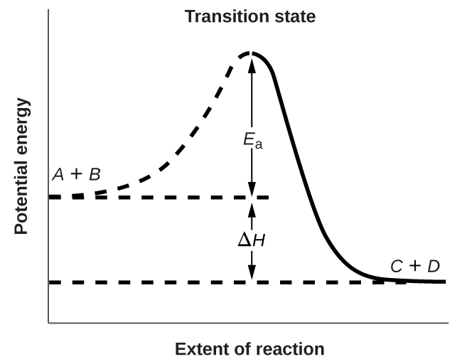
Figure \(\PageIndex{2}\): This graph shows the potential energy relationships for the reaction \(A+B⟶C+D\). The dashed portion of the curve represents the energy of the system with a molecule of A and a molecule of B present, and the solid portion the energy of the system with a molecule of C and a molecule of D present. The activation energy for the forward reaction is represented by Ea. The activation energy for the reverse reaction is greater than that for the forward reaction by an amount equal to ΔH. The peak represents the transition state.
Reactions with lower activation energies occur more quickly. If the activation energy is much larger than the average kinetic energy of the molecules, the reaction will be slow because only a small fraction of molecules will have enough energy to react. Conversely, if the activation energy is much smaller than the average kinetic energy, a greater fraction of molecules will possess the necessary energy, leading to frequent successful collisions and a faster reaction.
You previously encountered kinetic molecular theory (KMT) when studying gases. According to KMT, molecules in a sample have a range of kinetic energies, rather than a single fixed energy. At a given temperature, only a fraction of molecules have kinetic energy greater than the activation energy (Ea).
The relationship between activation energy and temperature on the fraction of molecules that can react is depicted visually in Figure \(\PageIndex{3}\):
- At a given temperature, a reaction with a lower activation energy will result in a larger fraction of molecules with enough energy to react. In Figure \(\PageIndex{3}\)(a) the opaque shaded area indicates the number of molecules with sufficient kinetic energy to react via the higher activation energy (Ea) reaction and this extends to include both the hatched and opaque shaded areas for a lower Ea reaction.
- Increasing temperature (T2 > T1) shifts the kinetic energy distribution so that more molecules have sufficient kinetic energy to exceed Ea. In Figure \(\PageIndex{3}\)(b) the number of molecules with sufficient energy to react increases from T1 (opaque shaded area) to T2 (hatched and opaque shaded areas). This explains why higher temperatures typically lead to faster reaction rates.
In everyday life, we know that food stored in a refrigerator lasts longer than food left at room temperature. This is because the lower temperature reduces the fraction of molecules with enough energy to react, slowing spoilage reactions. Similarly, cold-blooded animals (such as reptiles and insects) move more slowly on cold days because the biochemical reactions that power their muscles occur more slowly at lower temperatures.
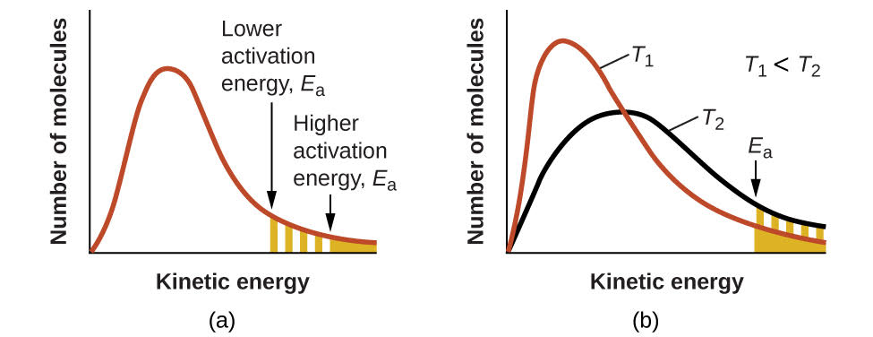
Figure \(\PageIndex{3}\): (a) As the activation energy of a reaction decreases, more molecules have this minimum energy, as shown by the shaded areas. (b) At a higher temperature, T2, more molecules have kinetic energies greater than Ea, as shown by the yellow shaded area.
Let's look at a reaction energy diagram in more detail. Consider the following reaction:
\[ \ce{CH3Br} + \ce{OH-} ⟶ \ce{CH3OH} + \ce{Br-} \nonumber\]
Figure \(\PageIndex{4}\) illustrates the change in potential energy as the reaction progresses from reactants to products. Since this reaction is exothermic, the products are lower in energy than the reactants. This also means that the activation energy for the forward reaction is lower than that for the reverse reaction.
As the reactants approach each other, repulsion between their electron clouds increases, causing kinetic energy to convert into potential energy, which slows their movement. If the collision occurs with sufficient energy, the reactants can reach the transition state, a high-energy, unstable species with partially broken and formed bonds.
In this reaction, the transition state consists of the central carbon atom surrounded by five other atoms. The carbon atom has three bonds to hydrogen atoms, a partial bond to bromine that is weakening, and a partial bond to oxygen that is forming. From the transition state, the reaction can proceed in either direction, towards products or back towards reactants.

Figure \(\PageIndex{4}\): Energy Profile of the reaction \( \ce{CH3Br} + \ce{OH-} ⟶ \ce{CH3OH} + \ce{Br-} \) . (Copyright; author via source Transition state theory. (2024, October 21). In Wikipedia. https://en.wikipedia.org/wiki/Transition_state_theory)
The Arrhenius Equation
The Arrhenius equation allows us to quantify the relationship between activation energy (Ea) and the rate constant (k) for a reaction:
\[k=Ae^{−E_a/RT} \label{Arrhenius} \]
where:
- \(R\) = universal gas constant (8.314 J mol-1 K-1)
- \(T\) = temperature (K)
- \(E_a\) = activation energy (J mol-1)
- \(A\) = frequency factor, a constant related to the frequency of collisions and their orientation (same units as k)
The Arrhenius equation relates the rate constant of a reaction (k) with the two key ideas of collision theory:
- The frequency factor (A) accounts for the number of collisions with the correct orientation.
- The exponential term \(e^{−E_a/RT}\) represents the fraction of molecules with enough kinetic energy to overcome the activation energy barrier.
The Arrhenius equation describes quantitatively much of what we have already discussed about reaction rates:
- Relationship between activation energy (Ea) and reaction rate: For two reactions at the same temperature, a larger Ea results in a smaller value of \(e^{−E_a/RT}\) , meaning fewer molecules have sufficient kinetic energy to react, resulting in a smaller rate constant (k) and a slower reaction rate. Conversely, a reaction with a smaller Ea has a larger fraction of molecules with sufficient energy, leading to a higher k and a faster reaction rate.
- Relationship between temperature (T) and reaction rate: Increasing temperature (T) results in a larger value of \(e^{−E_a/RT}\), meaning more molecules have sufficient kinetic energy to react, resulting in a larger rate constant (k) and a faster reaction rate.
As it connects the rate constant (k) of a reaction with temperature (T) and activation energy (Ea), the Arrhenius equation can be used to determine the activation energy barrier of a reaction by measuring the rate constant at different temperatures. This is simplified by taking the natural logarithm of both sides of the Arrhenius equation to produce a linear relationship:
\[\begin{align*}
\ln k&=\left(\dfrac{−E_a}{R}\right)\left(\dfrac{1}{T}\right)+\ln A\\
y&=mx+b
\end{align*} \nonumber \]
Plotting \(\ln k\) versus \(\dfrac{1}{T}\) produces a straight line. The slope of this line is \(\dfrac{-E_\ce{a}}{R}\), from which Ea may be determined. The y-intercept gives the value of \(\ln A\).
The table below provides rate constant () values at different temperatures for the decomposition of HI(g) into H₂(g) and I₂(g). Determine the activation energy () for this reaction.
\[\ce{2HI}(g)⟶\ce{H2}(g)+\ce{I2}(g) \nonumber \]
| T (K) | k (M-1s-1) |
|---|---|
| 555 | 3.52 × 10⁻⁷ |
| 575 | 1.22 × 10⁻⁶ |
| 645 | 8.59 × 10⁻⁵ |
| 700 | 1.16 × 10⁻³ |
| 781 | 3.95 × 10⁻² |
Solution
Values of \(\dfrac{1}{T}\) and ln k are:
| \(\mathrm{\dfrac{1}{T}\:(K^{−1})}\) | ln k |
|---|---|
| 1.80 × 10⁻³ | −14.860 |
| 1.74 × 10⁻³ | −13.617 |
| 1.55 × 10⁻³ | −9.362 |
| 1.43 × 10⁻³ | −6.759 |
| 1.28 × 10⁻³ | −3.231 |
Below is a graph of ln k versus \(\dfrac{1}{T}\). To determine the slope of the line, we need two values of ln k, which are determined from the line at two values of \(\dfrac{1}{T}\) (one near each end of the line is preferable). For example, the value of ln k determined from the line when \(\dfrac{1}{T}=1.25×10^{−3}\) is −2.593; the value when \(\dfrac{1}{T}=1.78×10^{−3}\) is −14.447.
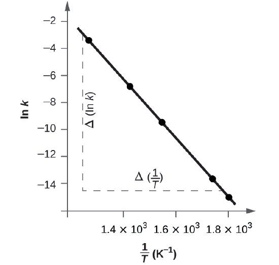
The slope of this line is given by the following expression:
\[\begin{align*}\ce{Slope}&=\dfrac{Δ(\ln k)}{Δ\left(\dfrac{1}{T}\right)}\\
&=\mathrm{\dfrac{(−14.447)−(−2.593)}{(1.78×10^{−3}\:K^{−1})−(1.25×10^{−3}\:K^{−1})}}\\
&=\mathrm{\dfrac{−11.854}{0.53×10^{−3}\:K^{−1}}=2.2×10^4\:K}\\
&=−\dfrac{E_\ce{a}}{R}
\end{align*} \nonumber \]
Thus:
\[ \begin{align*} E_\ce{a} &=\mathrm{−slope×\mathit R=−(−2.2×10^4\:K×8.314\: J\: mol^{−1}\:K^{−1})} \\[4pt] &=\mathrm{1.8×10^5\:J\: mol^{−1}} \end{align*} \nonumber \]
When only two temperature values and their corresponding rate constants are available, we can derive an equation that allows us to find the activation energy:
\[\ln k_1=\left(\dfrac{−E_\ce{a}}{R}\right)\left(\dfrac{1}{T_1}\right)+\ln A \nonumber \]
\[\ln k_2=\left(\dfrac{−E_\ce{a}}{R}\right)\left(\dfrac{1}{T_2}\right)+\ln A \nonumber \]
Subtracting these two equations eliminates lnA and gives:
\[\ln\left(\dfrac{k_2}{k_1}\right)=\dfrac{-E_\ce{a}}{R}\left(\dfrac{1}{T_2}−\dfrac{1}{T_1}\right) \label{Arrhenius2} \]
To see an example calculation, let's use the first entry and the last entry from the previous example :
| T (K) | k (M-1s-1) | \(\dfrac{1}{T}\:(K^{-1})\) | ln k |
|---|---|---|---|
| 555 | 3.52 × 10⁻⁷ | 1.80 × 10⁻³ | −14.860 |
| 781 | 3.95 × 10⁻² | 1.28 × 10⁻³ | −3.231 |
\[\ln\left(\dfrac{3.95 \times 10^{-2}M^{-1}s^{-1}}{3.52 \times 10^{-7}M^{-1}s^{-1}}\right)=\dfrac{-E_\ce{a}}{8.314 \dfrac{J}{mol\cdot K}}\left(\dfrac{1}{781K}−\dfrac{1}{555K}\right) \nonumber \]
\[11.63 = 6.27\times10^{-5}\dfrac{mol}{J}E_a \nonumber\]
\[E_a = 1.85 \times 10^5 J/mol \; \text{or}\; 185 kJ/mol\nonumber\]
This method is particularly useful when only a limited number of temperature-dependent rate constants are available for a reaction.
The rate constant for the rate of decomposition of N2O5 to NO and O2 in the gas phase is 1.66 M-1s-1 at 650 K and 7.39 M-1s-1 at 700 K:
\[\ce{2N2O5}(g)⟶\ce{4NO}(g)+\ce{3O2}(g) \nonumber \]
Calculate the activation energy for this decomposition.
- Answer
-
\[\ln\left(\dfrac{7.39\:M^{-1}s^{-1}}{1.66\:M^{-1}s^{-1}}\right)=\dfrac{-E_\ce{a}}{8.314 \dfrac{J}{mol\cdot K}}\left(\dfrac{1}{700\:K}−\dfrac{1}{650\:K}\right) \nonumber \]
Ea = 113,000 J/mol
Summary
Collision theory states that reactant molecules must collide with the correct orientation and sufficient energy to react. The activation energy is the minimum energy needed to reach the transition state, an unstable species between reactants and products with bonds partially broken and formed. The rate of a reaction is characterized by its rate constant, k, which is related to the activation energy barrier of the reaction, the temperature at which the reaction takes place, and the proportion of effective collisions.
Reaction energy diagrams illustrate how energy changes during a reaction. They visualize the energy of the transition state and the resulting activation energy barriers for both the forward and reverse reactions as well as the overall enthalpy change of the reaction.
The Arrhenius equation quantitatively describes how temperature and activation energy affect the rate constant. It allows the activation energy to be determined experimentally by measuring the rate constant at different temperatures.