6.4: Integrated Rate Laws

Learning Objectives

• Explain the form and function of an integrated rate law
• Perform integrated rate law calculations for zero-, first-, and second-order reactions
• Define half-life and carry out related calculations
• Identify the order of a reaction by plotting concentration vs. time data according to expected reaction orders

The rate laws we have seen so far relate reaction rates to reactant concentrations. Using calculus, the rate law can be integrated to derive an equation that relates reactant concentration to time. This can be done for any reaction order, but in this chapter we will focus on the integrated rate laws for zero-, first-, and second-order reactions.

Using the integrated rate law equations we can:

• Determine how much reactant or product is present after a given time.
• Estimate how long a reaction takes to reach a certain extent.
• Determine the reaction order of a reactant by plotting the change in concentration over time using the expected linear relationships for zero-, first-, and second-order reactions

Zero-Order Integrated Rate Law

A zero-order reaction is one in which the reaction rate is independent of reactant concentration. This means that the reaction proceeds at a constant rate, regardless of how much reactant is present. The rate law for a zero-order reaction is:

\[\ce{Rate}=-\dfrac{\Delta [A]}{\Delta t}=k[A]^0=k \nonumber \]

CHM135 does not require you to use calculus on assessments. However, we will derive the integrated rate laws here so you understand where they come from, after that you can simply use them. As shown above, the rate of a zero order reaction is independent of concentration:

 \[-\dfrac{d[A]}{dt}=k \nonumber\]

This equation can be rearranged to:

 \[ d[A] =-k \: dt \nonumber\]

By separating our variables and integrating our rate laws with respect \([A]\) on the left from \([A]_o\) to \([A]_t\) and with respect to \(t\) on the right from 0 to t, 

\[\int\limits_{[A]_o}^{[A]_t} \, d[A] = \int\limits_{0}^{t} -k\, dt \nonumber\]

we can generate the following linear relationships between concentration and time:

\[ [A]−[A]_0=−kt \nonumber\]

This is the integrated rate equation for a zero-order reaction, but it is typically rearranged to the following format:

\[ [A]=−kt+[A]_0 \nonumber\]

As it follows the general form of a linear equation:
\[ y =mx+b \notag \]

As shown in Figure \(\PageIndex{1}\) the plot of concentration versus time for a zero-order reaction is a straight line with a slope of −k and an intercept of [A]₀.

Figure \(\PageIndex{1}\) shows a plot of concentration versus time for a zero order reaction.

If the reaction order is known to be zero then we can use the integrated rate equation above to calculate changes in concentration over time. If the reaction order is unknown we can test whether a reaction is zero-order by plotting concentration versus time as a reaction proceeds. If this gives a linear relationship then the reaction order for that reactant is zero. When we do this we are modeling the reaction as if it were zero-order and seeing how the data fits this model. If it's not linear then we need to explore another model (maybe first-order or second-order). 

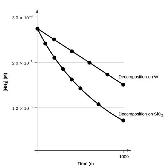
Figure \(\PageIndex{2}\) shows an example of this approach where experimental data for the decomposition of ammonia (NH₃) in the presence of two different materials at high temperatures are plotted together:

• Decomposition of ammonia (NH₃) on tungsten (W)
• Decomposition of ammonia (NH₃) on silica (SiO₂)

From the plot of [NH₃] versus time we can see that the decomposition on tungsten gives a straight line while that on silica does not, indicating the reaction order for NH₃ is zero when it involves tungsten but the reaction order of NH₃ is not zero when it involves silica.

Having a reaction order of zero feels a bit strange, but this is not unusual when a reaction involves a solid catalyst, which is the case here. Ammonia gas diffuses onto the surface of the solid tungsten first and then once there they react. Once the surface is fully occupied, adding more ammonia does not increase the rate, leading to zero-order kinetics.  From the slope of the line for the zero-order decomposition, the rate constant can be determined:

\[\ce{slope}=−k=\mathrm{1.3110^{−6}\:mol/L/s} \nonumber \]

Figure \(\PageIndex{2}\): The decomposition of NH₃ in the presence of tungsten (W) surface is a zero-order reaction, whereas, with quartz (SiO₂), the reaction is first-order.

 

First-Order Integrated Rate Law

The rate law for a first-order reaction is:

\[\ce{Rate}=-\dfrac{\Delta [A]}{\Delta t}=k[A]^1 \nonumber \]

Changing deltas to differentials,

\[\ -\dfrac{d[A]}{dt} =k [A] \nonumber \]

then rearranging the equation to separate the variables \([A]\) and \(t\),

\[\ \dfrac{1}{[A]} d[A]=-k \: dt \nonumber \]

we can integrate with respect to \([A]\) on the left from \([A]_o\) to \([A]_t\) and with respect to \(t\) on the right from 0 to t:

\[\int\limits_{[A]_o}^{[A]_t} \dfrac{1}{[A]}\, d[A] = \int\limits_{0}^{t} -k\, dt \nonumber\]

This gives us the first-order integrated rate law, which provides a linear expression for changes in reactant concentration as a function of time,

\[ ln[A]-\ln[A]_0=−kt \nonumber\]

or,

\[ \ln\left(\dfrac{[A]_t}{[A]_0}\right)=−kt \nonumber\]

which can be rearranged into the form of a linear equation:

\[ ln[A]=−kt+\ln[A]_0 \nonumber\]
\[ y=mx+b \notag \]

This is the integrated rate expression for a first-order reaction, and, similar to the zero-order reactions in the section above, this equation allows us to calculate the concentration of A at any time ([A]_t), given the initial concentration ([A]₀), the rate constant (k) and the elapsed time (t).

For a first-order reaction, a plot of \(ln[A]\) versus \(t\) yields a straight line with a slope of \(−k\) and an intercept of \( ln[A]_0\). If data plotted this way does not result in a straight line, the reaction is not first order in \(A\).

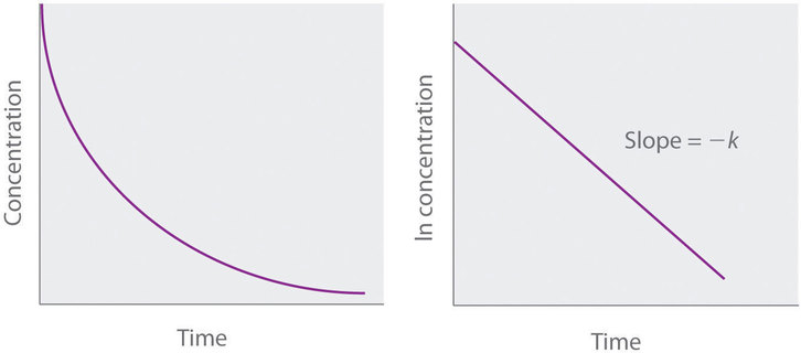
Figure \(\PageIndex{3}\): Graphs of a first-order reaction. The expected shapes of the curves for plots of reactant concentration versus time (left) and the natural logarithm of reactant concentration versus time (right) for a first-order reaction.

Example \(\PageIndex{1}\): The Integrated Rate Law for a First-Order Reaction

The rate constant for the first-order decomposition of cyclobutane, \(\ce{C4H8}\) at 500 °C is 9.2 × 10⁻³ s⁻¹:

\[\ce{C4H8⟶2C2H4} \nonumber \]

How long will it take for 80.0% of a sample of C₄H₈ to decompose?

Solution

Since we need to find time, we use the integrated form of the rate law :

\[\ln\left(\dfrac{[A]_0}{[A]}\right)=kt \nonumber \]

The initial concentration of C₄H₈, [A]₀, is not provided, we know that 80.0% of the sample has decomposed,, meaning that 20.0% remains:

[A]_t = 0.200[A]₀

Rearranging the rate law to isolate t and substituting the provided quantities yields:

\[\begin{align*}
t&=\ln\dfrac{[A]_0}{[0.200[A]_0]}×\dfrac{1}{k}\\[4pt]
&=\mathrm{\ln\dfrac{1}{0.200}×\dfrac{1}{9.2×10^{−3}\:s^{−1}}}\\[4pt]
&=\mathrm{1.609×\dfrac{1}{9.2×10^{−3}\:s^{−1}}}\\[4pt]
&=\mathrm{1.7×10^2\:s}
\end{align*} \nonumber \]

Exercise \(\PageIndex{1}\)

Iodine-131 is a radioactive isotope that is used to diagnose and treat some forms of thyroid cancer. Iodine-131 decays to xenon-131 according to the equation:

\[\textrm{I-131 ⟶ Xe-131 + electron} \nonumber \]

The decay is first-order with a rate constant of 0.138 d⁻¹. All radioactive decay is first order. How many days will it take for 90% of the iodine−131 in a 0.500 M solution of this substance to decay to Xe-131?

Answer

16.7 days

Example \(\PageIndex{2}\): Determination of Reaction Order by Graphing

Demonstrate that the decomposition of H₂O₂ follows a first-order rate law by graphing ln[H₂O₂] versus time. Determine the rate constant for the rate of decomposition of H₂O₂.

Time (h)	[H2O2] (M)	ln[H2O2]
0	1.000	0.0
6.00	0.500	−0.693
12.00	0.250	−1.386
18.00	0.125	−2.079
24.00	0.0625	−2.772

Solution

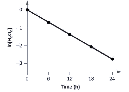
The linear relationship between the ln[H₂O₂] and time shows that the decomposition of hydrogen peroxide is a first-order reaction.

The rate constant for a first-order reaction is equal to the negative of the slope of the plot of ln[H₂O₂] versus time where:

\[\ce{slope}=\dfrac{\textrm{change in }y}{\textrm{change in }x}=\dfrac{Δy}{Δx}=\dfrac{Δ\ln[\ce{H2O2}]}{Δt} \nonumber \]

To determine the slope of the line, we need two values of ln[H₂O₂] at different values of t (one near each end of the line is preferable). For example, the value of ln[H₂O₂] when t is 6.00 h is −0.693; the value when t = 12.00 h is −1.386:

\[\begin{align*}
\ce{slope}&=\mathrm{\dfrac{−1.386−(−0.693)}{12.00\: h−6.00\: h}}\\[4pt]
&=\mathrm{\dfrac{−0.693}{6.00\: h}}\\[4pt]
&=\mathrm{−1.155×10^{−2}\:h^{−1}}\\[4pt]
k&=\mathrm{−slope=−(−1.155×10^{−1}\:h^{−1})=1.155×10^{−1}\:h^{−1}}
\end{align*} \nonumber \]

Exercise \(\PageIndex{2}\)

Graph the following data to determine whether the reaction \(A⟶B+C\) is first order.

Data for the reaction \(A⟶B+C\)

Trial	Time (s)	[A]
1	4.0	0.220
2	8.0	0.144
3	12.0	0.110
4	16.0	0.088
5	20.0	0.074

Answer

The plot of ln[A] vs. t is not a straight line. The equation is not first order:

 

Second-Order Integrated Rate Law

A reaction that is second-order overall can occur in two ways:

• One reactant with a reaction order of 2: rate = k[A]²
• Two reactants each with a reaction order of 1: rate = k[A][B]

In this section, we are focussing on the first case, which assesses whether the reaction order of a single reactant is second order. However, in the CHM135 laboratory we will explore how the reaction orders of multi-component rate laws can be determined.

The rate law for a second-order reaction is:

\[\ce{rate}=-\dfrac{\Delta [A]}{\Delta t}=k[A]^2 \nonumber \]

Changing deltas to differentials,

\[\ -\dfrac{d[A]}{dt} =k [A]^2 \nonumber \]

then rearranging the equation to separate the variables \([A]\) and \(t\),

\[\ \dfrac{1}{[A]^2}  \: d[A]=-k \: dt \nonumber \]

we can integrate with respect to \([A]\) on the left from \([A]_o\) to \([A]_t\) and with respect to \(t\) on the right from 0 to t:

\[\int\limits_{[A]_o}^{[A]_t} \dfrac{1}{[A]^2}\, d[A] = \int\limits_{0}^{t} -k\, dt \nonumber\]

This gives us the second-order integrated rate law, which provides a linear expression for changes in reactant concentration as a function of time:

\[-(\dfrac{1}{[A]}-\dfrac{1}{[A]_0})=-kt \label{int2nd} \]

The integrated rate law for the second-order reaction can be rewritten in the form of a linear equation:

\[\begin{align*}
\dfrac{1}{[A]}&=kt+\dfrac{1}{[A]_0}\\[4pt]
y&=mx+b
\end{align*} \nonumber \]

For a second-order reaction, a plot of \(\dfrac{1}{[A]}\) versus \(t\) yields a straight line with a slope of \(k\) and an intercept of \(\dfrac{1}{[A]_0}\). If this plot is not a straight line, the reaction is not second order.

Example \(\PageIndex{3}\): The Integrated Rate Law for a Second-Order Reaction

The reaction of butadiene gas (C₄H₆) with itself produces C₈H₁₂ gas as follows:

\[\ce{2C4H6}(g)⟶\ce{C8H12(g)} \nonumber \]

The reaction is second order with a rate constant equal to 5.76 × 10⁻² L/mol/min under certain conditions. If the initial concentration of butadiene is 0.200 M, what is the concentration remaining after 10.0 min?

Solution

We use the integrated form of the rate law to answer questions regarding time. For a second-order reaction, we have:

\[\dfrac{1}{[A]}=kt+\dfrac{1}{[A]_0} \nonumber \]

\[\begin{align*}
\dfrac{1}{[A]}&=\mathrm{(5.76×10^{−2}\:L\: mol^{−1}\:min^{−1})(10\:min)+\dfrac{1}{0.200\:M}}\\[4pt]
\dfrac{1}{[A]}&=\mathrm{(5.76×10^{−1}\:M^{−1})+5.00\:M^{−1}}\\[4pt]
\dfrac{1}{[A]}&=\mathrm{5.58\:M^{−1}}\\[4pt]
[A]&=\mathrm{1.79×10^{−1}\:M}
\end{align*} \nonumber \]

Therefore 0.179 mol/L of butadiene remain at the end of 10.0 min, compared to the 0.200 mol/L that was originally present.

Exercise \(\PageIndex{3}\)

Using the reaction in Example \(\PageIndex{4}\) with an initial concentration of butadiene is 0.0200 M, what is the concentration remaining after 20.0 min?

Answer

0.0195 mol/L

 

Example \(\PageIndex{4}\): Determination of Reaction Order by Graphing

Test the data given to show whether the dimerization of C₄H₆ is a first- or a second-order reaction.

Solution

Solutions to Example 12.4.4

Time (s)	[C4H6] (M)
0	1.00 × 10^−2
1600	5.04 × 10^−3
3200	3.37 × 10^−3
4800	2.53 × 10^−3
6200	2.08 × 10^−3

To distinguish a first-order reaction from a second-order reaction, we plot ln[C₄H₆] versus t and compare it with a plot of \(\mathrm{\dfrac{1}{[C_4H_6]}}\) versus t. The values needed for these plots follow.

Time (s)	\(\dfrac{1}{[\ce{C4H6}]}\:(M^{−1})\)	ln[C4H6]
0	100	−4.605
1600	198	−5.289
3200	296	−5.692
4800	395	−5.978
6200	481	−6.175

As you can see, the plot of ln[C₄H₆] versus t is not linear, therefore the reaction is not first order. The plot of \(\dfrac{1}{[\ce{C4H6}]}\) versus t is linear, indicating that the reaction is second order.

These two graphs show first- and second-order plots for the dimerization of C₄H₆. Since the first-order plot (left) is not linear, we know that the reaction is not first order. The linear trend in the second-order plot (right) indicates that the reaction follows second-order kinetics.

 

Exercise \(\PageIndex{4}\)

Does the following data fit a second-order rate law?

Data for second-order rate law

Trial	Time (s)	[A] (M)
1	5	0.952
2	10	0.625
3	15	0.465
4	20	0.370
5	25	0.308
6	35	0.230

 

Answer

Yes. The plot of \(\dfrac{1}{[A]}\) vs. t is linear:

 

 

The Half-Life of a Reaction

The half-life of a reaction (t_1/2) is the time required for the reactant concentration to decrease by half. In each succeeding half-life, half of the remaining concentration of the reactant is consumed. For a first-order reaction, the half-life remains constant and does not depend on the starting concentration.

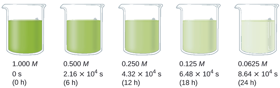
For example, the decomposition of hydrogen peroxide (H₂O₂) follows first-order kinetics. Figure \(\PageIndex{4}\) shows its concentration decreasing over time in a series of four half-lives:

•     First half-life: [H₂O₂] decreases from 1.00 M to 0.500 M
•     Second half-life: [H₂O₂] decreases from 0.500 M to 0.250 M
•     Third half-life: [H₂O₂] decreases from 0.250 M to 0.125 M
•     Fourth half-life: [H₂O₂] decreases from 0.125 M to 0.0625 M

From this plot, we can see that each half-life is 6 hours, confirming that the half-life of a first-order reaction remains constant over time.

Figure \(\PageIndex{4}\): The decomposition of H₂O₂ is a first-order reaction.  At a particular temperature, the half-life of the reaction is 6 hours, meaning that half of the  H₂O₂ decomposes every 6 hours.  This plot shows 4 successive half-lives where the [H₂O₂] decreases from 1 M to 0.5 M in the first, 0.500 M to 0.250 M in the second, 0.250 M to 0.125 M in the third and 0.125 M to 0.0625 M in the fourth.

The half-life of a first-order reaction can be derived from its integrated rate law:

\[\ln\dfrac{[A]_0}{[A]_t}=kt \nonumber \]

Solving for t:

\[t=\dfrac{ln\dfrac{[A]_0}{[A]_t}}{k}\nonumber \]

Since half-life is the time when [A] is half of its initial value, we substitute [A]_t = 1/2[A]₀​ and set t = t_1/2​:

\[t_{1/2}=\dfrac{ln\dfrac{[A]_0}{\dfrac{1}{2}[A]_0}}{k}\nonumber \]

Simplifying:

\[t_{1/2}=\dfrac{\ln2}{k}=\dfrac{0.693}{k}\nonumber \]

This equation shows that the half-life of a first-order reaction is independent of reactant concentration and depends only on the rate constant k.  We can also see that the half-life of a first-order reaction is inversely proportional to the rate constant k. A fast reaction (larger k) will have a shorter half-life; a slow reaction (smaller k) will have a longer half-life.  This relationship makes half-life calculations particularly useful in fields like pharmacology (drug metabolism) and nuclear chemistry (radioactive decay), where processes are often first-order and knowing how long a substance persists is essential.

Example \(\PageIndex{5}\): Calculation of a First-order Rate Constant using Half-Life

Calculate the rate constant for the first-order decomposition of hydrogen peroxide in water at 40 °C, using the data given below:

The decomposition of H₂O₂ \(\ce{(2H2O2⟶2H2O + O2)}\) at 40 °C is illustrated. The intensity of the colour symbolizes the concentration of H₂O₂ at the indicated times; H₂O₂ is actually colourless.

Solution

The half-life for the decomposition of H₂O₂ is 2.16 × 10⁴ s:

\[\begin{align*}
t_{1/2}&=\dfrac{0.693}{k}\\[4pt]
k&=\dfrac{0.693}{t_{1/2}}=\dfrac{0.693}{2.16×10^4\:\ce s}=3.21×10^{−5}\:\ce s^{−1}
\end{align*} \nonumber \]

Exercise \(\PageIndex{5}\)

The first-order radioactive decay of iodine-131 exhibits a rate constant of 0.138 d⁻¹. What is the half-life for this decay?

Answer

5.02 d.

 

The half-life (t_1/2) of a zero-order reaction can be determined using the zero-order integrated rate law:

\[[A]=−kt+[A]_0 \nonumber \]

Substituting t = t_1/2​ and [A]_t = 1/2[A]₀:

\[\begin{align*}
\dfrac{[A]_0}{2}&=−kt_{1/2}+[A]_0\\[4pt]
kt_{1/2}&=\dfrac{[A]_0}{2}\\[4pt]
t_{1/2}=\dfrac{[A]_0}{2k}
\end{align*} \nonumber \]

This equation demonstrates that the half-life of a zero-order reaction depends on the initial concentration ([A]₀) and that as the reaction proceeds, the half-life decreases. This might seem strange, if the half-life is decreases... does that mean the rate of the reaction is increasing as time going on? No, that is (obviously) possible. In a zero-order reaction the rate of the reaction is unchanged with reactant concentration and so as the reaction proceeds the half-life gets shorter because there is simply less material present and so it will not take as long to half that smaller amount as the rate is not changing.

The half-life (t_1/2​) of a second-order reaction can be determined using the second-order integrated rate law:

\[\dfrac{1}{[A]}=kt+\dfrac{1}{[A]_0} \nonumber \]

Substituting t = t_1/2​ and [A]_t = 1/2[A]₀:

\(\begin{align*}
\dfrac{1}{[A]}−\dfrac{1}{[A]_0}&=kt\\[4pt]
\dfrac{1}{\dfrac{1}{2}[A]_0}−\dfrac{1}{[A]_0}&=kt_{1/2}\\[4pt]
2[A]_0−\dfrac{1}{[A]_0}&=kt_{1/2}\\[4pt]
\dfrac{1}{[A]_0}&=kt_{1/2}\\[4pt]
t_{1/2}&=\dfrac{1}{k[A]_0}
\end{align*}\nonumber \)

This equation shows that the half-life of a second-order reaction is inversely proportional to the initial concentration ([A]₀) and so as the reaction proceeds, the half-life increases. This increase in half-life means the reaction is proceeding at a slower rate as the reactant is consumed.

Comparing Zero-, First-, and Second-Order Reactions

The following table summarizes the key differences between zero-, first-, and second-order reactions:

Table \(\PageIndex{1}\): Summary of Rate Laws for Zero-, First-, and Second-Order Reactions

	Zero-Order	First-Order	Second-Order
Rate law	rate = k	rate = k[A]	rate = k[A]^2
Units of k	M s^−1	s^−1	M^−1 s^−1
Integrated rate law	[A]t = −kt + [A]0	ln[A]t = −kt + ln[A]0	\(\dfrac{1}{[A]_t}=kt+\left(\dfrac{1}{[A]_0}\right)\)
Graph for linear fit	[A] vs. t	ln[A] vs. t	\(\dfrac{1}{[A]}\) vs. t
Slope in graph	k = −slope	k = −slope	k = +slope
Half-life	\(t_{1/2}=\dfrac{[A]_0}{2k}\)	\(t_{1/2}=\dfrac{0.693}{k}\)	\(t_{1/2}=\dfrac{1}{[A]_0k}\)

Summary

Rate laws describe how the rate of a reaction depends on reactant concentration. Reaction orders and the rate constant within the rate law can be determined using the method of initial rates or graphical analysis of concentration vs. time data.

Integrated rate laws describe how reactant concentrations change over time and are derived by integrating the rate laws.

The half-life of a reaction is the time required to decrease the amount of a given reactant by one-half. In a zero-order reaction, the half-life decreases as the reaction proceeds. In a first-order reaction, the half-life is constant and does not depend on concentration. In a second-order reaction, the half-life increases as the reaction proceeds.