
6.3: Rate Laws
- Page ID
- 499146

\( \newcommand{\vecs}[1]{\overset { \scriptstyle \rightharpoonup} {\mathbf{#1}} } \)
\( \newcommand{\vecd}[1]{\overset{-\!-\!\rightharpoonup}{\vphantom{a}\smash {#1}}} \)
\( \newcommand{\dsum}{\displaystyle\sum\limits} \)
\( \newcommand{\dint}{\displaystyle\int\limits} \)
\( \newcommand{\dlim}{\displaystyle\lim\limits} \)
\( \newcommand{\id}{\mathrm{id}}\) \( \newcommand{\Span}{\mathrm{span}}\)
( \newcommand{\kernel}{\mathrm{null}\,}\) \( \newcommand{\range}{\mathrm{range}\,}\)
\( \newcommand{\RealPart}{\mathrm{Re}}\) \( \newcommand{\ImaginaryPart}{\mathrm{Im}}\)
\( \newcommand{\Argument}{\mathrm{Arg}}\) \( \newcommand{\norm}[1]{\| #1 \|}\)
\( \newcommand{\inner}[2]{\langle #1, #2 \rangle}\)
\( \newcommand{\Span}{\mathrm{span}}\)
\( \newcommand{\id}{\mathrm{id}}\)
\( \newcommand{\Span}{\mathrm{span}}\)
\( \newcommand{\kernel}{\mathrm{null}\,}\)
\( \newcommand{\range}{\mathrm{range}\,}\)
\( \newcommand{\RealPart}{\mathrm{Re}}\)
\( \newcommand{\ImaginaryPart}{\mathrm{Im}}\)
\( \newcommand{\Argument}{\mathrm{Arg}}\)
\( \newcommand{\norm}[1]{\| #1 \|}\)
\( \newcommand{\inner}[2]{\langle #1, #2 \rangle}\)
\( \newcommand{\Span}{\mathrm{span}}\) \( \newcommand{\AA}{\unicode[.8,0]{x212B}}\)
\( \newcommand{\vectorA}[1]{\vec{#1}} % arrow\)
\( \newcommand{\vectorAt}[1]{\vec{\text{#1}}} % arrow\)
\( \newcommand{\vectorB}[1]{\overset { \scriptstyle \rightharpoonup} {\mathbf{#1}} } \)
\( \newcommand{\vectorC}[1]{\textbf{#1}} \)
\( \newcommand{\vectorD}[1]{\overrightarrow{#1}} \)
\( \newcommand{\vectorDt}[1]{\overrightarrow{\text{#1}}} \)
\( \newcommand{\vectE}[1]{\overset{-\!-\!\rightharpoonup}{\vphantom{a}\smash{\mathbf {#1}}}} \)
\( \newcommand{\vecs}[1]{\overset { \scriptstyle \rightharpoonup} {\mathbf{#1}} } \)
\(\newcommand{\longvect}{\overrightarrow}\)
\( \newcommand{\vecd}[1]{\overset{-\!-\!\rightharpoonup}{\vphantom{a}\smash {#1}}} \)
\(\newcommand{\avec}{\mathbf a}\) \(\newcommand{\bvec}{\mathbf b}\) \(\newcommand{\cvec}{\mathbf c}\) \(\newcommand{\dvec}{\mathbf d}\) \(\newcommand{\dtil}{\widetilde{\mathbf d}}\) \(\newcommand{\evec}{\mathbf e}\) \(\newcommand{\fvec}{\mathbf f}\) \(\newcommand{\nvec}{\mathbf n}\) \(\newcommand{\pvec}{\mathbf p}\) \(\newcommand{\qvec}{\mathbf q}\) \(\newcommand{\svec}{\mathbf s}\) \(\newcommand{\tvec}{\mathbf t}\) \(\newcommand{\uvec}{\mathbf u}\) \(\newcommand{\vvec}{\mathbf v}\) \(\newcommand{\wvec}{\mathbf w}\) \(\newcommand{\xvec}{\mathbf x}\) \(\newcommand{\yvec}{\mathbf y}\) \(\newcommand{\zvec}{\mathbf z}\) \(\newcommand{\rvec}{\mathbf r}\) \(\newcommand{\mvec}{\mathbf m}\) \(\newcommand{\zerovec}{\mathbf 0}\) \(\newcommand{\onevec}{\mathbf 1}\) \(\newcommand{\real}{\mathbb R}\) \(\newcommand{\twovec}[2]{\left[\begin{array}{r}#1 \\ #2 \end{array}\right]}\) \(\newcommand{\ctwovec}[2]{\left[\begin{array}{c}#1 \\ #2 \end{array}\right]}\) \(\newcommand{\threevec}[3]{\left[\begin{array}{r}#1 \\ #2 \\ #3 \end{array}\right]}\) \(\newcommand{\cthreevec}[3]{\left[\begin{array}{c}#1 \\ #2 \\ #3 \end{array}\right]}\) \(\newcommand{\fourvec}[4]{\left[\begin{array}{r}#1 \\ #2 \\ #3 \\ #4 \end{array}\right]}\) \(\newcommand{\cfourvec}[4]{\left[\begin{array}{c}#1 \\ #2 \\ #3 \\ #4 \end{array}\right]}\) \(\newcommand{\fivevec}[5]{\left[\begin{array}{r}#1 \\ #2 \\ #3 \\ #4 \\ #5 \\ \end{array}\right]}\) \(\newcommand{\cfivevec}[5]{\left[\begin{array}{c}#1 \\ #2 \\ #3 \\ #4 \\ #5 \\ \end{array}\right]}\) \(\newcommand{\mattwo}[4]{\left[\begin{array}{rr}#1 \amp #2 \\ #3 \amp #4 \\ \end{array}\right]}\) \(\newcommand{\laspan}[1]{\text{Span}\{#1\}}\) \(\newcommand{\bcal}{\cal B}\) \(\newcommand{\ccal}{\cal C}\) \(\newcommand{\scal}{\cal S}\) \(\newcommand{\wcal}{\cal W}\) \(\newcommand{\ecal}{\cal E}\) \(\newcommand{\coords}[2]{\left\{#1\right\}_{#2}}\) \(\newcommand{\gray}[1]{\color{gray}{#1}}\) \(\newcommand{\lgray}[1]{\color{lightgray}{#1}}\) \(\newcommand{\rank}{\operatorname{rank}}\) \(\newcommand{\row}{\text{Row}}\) \(\newcommand{\col}{\text{Col}}\) \(\renewcommand{\row}{\text{Row}}\) \(\newcommand{\nul}{\text{Nul}}\) \(\newcommand{\var}{\text{Var}}\) \(\newcommand{\corr}{\text{corr}}\) \(\newcommand{\len}[1]{\left|#1\right|}\) \(\newcommand{\bbar}{\overline{\bvec}}\) \(\newcommand{\bhat}{\widehat{\bvec}}\) \(\newcommand{\bperp}{\bvec^\perp}\) \(\newcommand{\xhat}{\widehat{\xvec}}\) \(\newcommand{\vhat}{\widehat{\vvec}}\) \(\newcommand{\uhat}{\widehat{\uvec}}\) \(\newcommand{\what}{\widehat{\wvec}}\) \(\newcommand{\Sighat}{\widehat{\Sigma}}\) \(\newcommand{\lt}{<}\) \(\newcommand{\gt}{>}\) \(\newcommand{\amp}{&}\) \(\definecolor{fillinmathshade}{gray}{0.9}\)- Explain the form and function of a rate law
- Use rate laws to calculate reaction rates
- Use rate and concentration data to identify reaction orders and derive rate laws
Form of the Rate Law and Reaction Orders
The rate of a reaction depends on the concentrations of reactants. A rate law is a mathematical expression that describes this relationship:
\[\ce{rate}=k[A]^m[B]^n[C]^p… \nonumber \]
where [A], [B], and [C] represent the concentrations of the reactants, typically expressed in molarity. k is the rate constant, which does not depend on reactant concentrations but varies with temperature. The exponents m, n, and p are the reaction orders with respect to each reactant. Reaction orders are typically positive integers, and they define how the concentration of each reactant influences the reaction rate. All components of the rate law must be determined experimentally.
The exponents in the rate law determine the reaction order with respect to each reactant. Consider a reaction with the rate law:
\[\ce{rate}=k[A]^m[B]^n \nonumber \]
- If m is 1, the reaction is first order in A; if m is 2, the reaction is second order in A;
- If n is 1, the reaction is first order in B; if n is 2, the reaction is second order in B;
- If m or n is zero, the reaction is zero order in A or B, respectively (the rate is unaffected by the reactant concentration)
The overall reaction order is the sum of the individual orders. For example, if m = 1 and n = 1, the overall order of the reaction is second order (m + n = 2).
Consider the decomposition of hydrogen peroxide:
\[\ce{2H2O2}(aq)⟶\ce{2H2O}(l)+\ce{O2}(g) \nonumber \]
Experimental data shows that the rate law for this reaction is:
\[\ce{rate}=k[\ce{H2O2}] \nonumber \]
Since the exponent is 1, the reaction is first order in H2O2 and first order overall. The rate is directly proportional to ; if the concentration doubles, the reaction rate also doubles.
An experiment shows that the reaction of nitrogen dioxide with carbon monoxide:
\[\ce{NO2}(g)+\ce{CO}(g)⟶\ce{NO}(g)+\ce{CO2}(g) \nonumber \]
is second order in NO2 and zero order in CO at 100 °C.
a) What is the rate law for the reaction?
b) How does doubling [NO2] affect the rate?
c) How does halving [CO] affect the rate?
Solution
a) The reaction will have the form:
\[\ce{rate}=k[\ce{NO2}]^m[\ce{CO}]^n \nonumber \]
The reaction is second order in NO2; thus m = 2. The reaction is zero order in CO; thus n = 0. The rate law is:
\[\ce{rate}=k[\ce{NO2}]^2[\ce{CO}]^0=k[\ce{NO2}]^2 \nonumber \]
Remember that a number raised to the zero power is equal to 1, thus [CO]0 = 1, which is why we can simply drop the concentration of CO from the rate equation: the rate of reaction is solely dependent on the concentration of NO2. When we consider rate mechanisms later in this chapter, we will explain how a reactant’s concentration can have no effect on a reaction despite being involved in the reaction.
b) Since the reaction is second order in NO2, doubling the concentration increases the rate by a factor of 4.
c) The reaction is zero order in CO, so halving the concentration will not affect the rate.
The rate law for the reaction:
\[\ce{H2}(g)+\ce{2NO}(g)⟶\ce{N2O}(g)+\ce{H2O}(g) \nonumber \]
has been experimentally determined to be rate = k[NO]2[H2]. What are the orders with respect to each reactant, and what is the overall order of the reaction?
- Answer
-
- order in NO = 2;
- order in H2 = 1;
- overall order = 3
The reaction between methanol (CH3OH) and ethyl acetate (CH3CH2OCOCH3) follows the equation:
\[\ce{CH3OH + CH3CH2OCOCH3 ⟶ CH3OCOCH3 + CH3CH2OH} \nonumber \]
Under certain conditions, the experimentally determined rate law is:
\[\ce{rate}=k[\ce{CH3OH}] \nonumber \]
What is the order of reaction with respect to methanol and ethyl acetate, and what is the overall order?
- Answer
-
- order in CH3OH = 1;
- order in CH3CH2OCOCH3 = 0;
- overall order = 1
These examples illustrate an important point: reaction orders cannot be determined from the coefficients in the balanced reaction. Reaction orders must be determined experimentally. How do we determine the orders in the rate law? In CHM 135, we will discuss two methods, starting with the method of initial rates.
Method of Initial Rates
The method of initial rates involves measuring the initial rate of a reaction under different reactant concentrations to see how the rate varies. These experiments typically involve changing the concentration of one reactant at a time to see how the rate of the reaction varies with this change.
Consider the reaction and A and B:
\[A + B \rightarrow products \nonumber \]
With the following experimental data collected over three runs:
| Run | [A] (M) | [B] (M) | Rate (M/s) |
|---|---|---|---|
| 1 | 0.0100 | 0.0100 | 0.0347 |
| 2 | 0.0200 | 0.0100 | 0.0694 |
| 3 | 0.0200 | 0.0200 | 0.2776 |
The rate law for this reaction will take the following form:
\[ \text{rate} = k [A]^m [B]^n \nonumber\]
Now we need to use the data to determine the values of k, m, and n. We will explore two different ways to approach this analysis.
Finding Reaction Orders By Inspection:
By comparing data sets where one reactant is held constant, we can determine the reaction order for each reactant:
- Finding the order with respect to A:
Comparing Runs 1 and 2, [B] is unchanged (0.0100 M), so any change in rate is due to [A].
Since [A] doubles and the rate also doubles, the reaction is first order in A (m = 1).
- Finding the order with respect to B:
Comparing Runs 2 and 3, [A] is unchanged (0.0200M), so any change in rate is due to [B].
Since [B] doubles and the rate increases by a factor of 4, the reaction is second order in B (n = 2).
This gives the rate law:
\[ \text{rate} = k [A] [B]^2 \nonumber\]
Mathematical Approach:
The reaction orders can also be determined mathematically by dividing two rate equations:
- Finding the order with respect to A, m, using the ratio of the rate laws for Runs 2 and 1:
\[ \frac{\text{rate}_i}{\text{rate}_j} = \frac{k [A]_i^m [B]_i^n}{k [A]_j^m [B]_j^n}\nonumber \]
\[ \frac{0.0694\,\text{M/s}}{0.0347\, \text{M/s}} = \frac{\cancel{k} (0.0200\,\text{M})^m \cancel{(0.0100\,\text{M})^n}}{\cancel{k} (0.0100\,\text{M})^m \cancel{(0.0100\,\text{M})^n}}\nonumber \]
\[ 2 = 2^m\nonumber \]
In this case we can solve for m by inspection, m = 1, confirming the reaction is first order with respect to A.
- Finding the order with respect to B, n, using the ratio of the rate laws for Runs 3 and 2:
\[ \frac{0.2776\, \text{M/s}}{0.0694\, \text{M/s}} = \frac{\cancel{k} (0.0200\,\text{M})^m (0.0200\,\text{M})^n}{\cancel{k} (0.0200\,\text{M})^m (0.0100\,\text{M})^n} \nonumber\]
\[ 4 = 2^n \nonumber \]
We might also be able to solve this equation by inspection, but in case the math is not so simple, or we want to double check, we can solve for the exponent by taking the logarithm of both sides (in this case we chose the log10):
\[\log(4)=\log(2^n) \nonumber\]
Then we can use the rules for manipulating logarithms to solve for n:
\[\log(4)=n\log(2) \nonumber\]
\[n=\dfrac{\log(4)}{\log(2)}=2 \nonumber\]
We find n = 2, confirming the reaction is second order with respect to B.
\[ \text{rate} = k [A][B]^{2} \nonumber \]
The rate law indicates that the reaction is 1st order in A, 2nd order in B, and 3rd order overall.
Determining the rate constant
The rate constant k can be calculated by substituting any experimental data set into the rate law. Using Run 1:
\[ 0.0347 \,M/s = k (0.0100 \, M)(0.0100 \, M)^{2} \nonumber \]
Solving for k:
\[ k = \dfrac{0.0347 \,M/s} {(0.0100 \, M)(0.0100 \, M)^2} = 3.47 \times 10^{5} \, M^{-2} s^{-1} \nonumber \]
Pay careful attention to the units of k as the units will change with the order of the reaction.
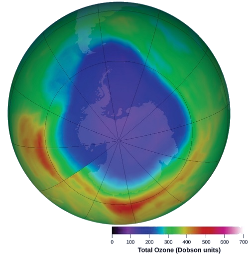
Ozone in the upper atmosphere is depleted by reactions with nitrogen oxides, contributing to the formation of the ozone hole over Antarctica (Figure \(\PageIndex{1}\)). The rates of these reactions are critical in assessing their environmental impact.
One such reaction is the combination of nitric oxide (NO) with ozone (O3):
\[\ce{NO}(g)+\ce{O3}(g)⟶\ce{NO2}(g)+\ce{O2}(g) \nonumber \]
This reaction has been studied in the laboratory, and the following initial rate data were determined at 25 °C.
| Trial | \([\ce{NO}]\) (M) | \([\ce{O3}]\) (M) | \(\dfrac{Δ[\ce{NO2}]}{Δt}\:\mathrm{(M\:s^{−1})}\) |
|---|---|---|---|
| 1 | 1.00 × 10⁻⁶ | 3.00 × 10⁻⁶ | 6.60 × 10⁻⁵ |
| 2 | 1.00 × 10⁻⁶ | 6.00 × 10⁻⁶ | 1.32 × 10⁻⁴ |
| 3 | 1.00 × 10⁻⁶ | 9.00 × 10⁻⁶ | 1.98 × 10⁻⁴ |
| 4 | 2.00 × 10⁻⁶ | 9.00 × 10⁻⁶ | 3.96 × 10⁻⁴ |
| 5 | 3.00 × 10⁻⁶ | 9.00 × 10⁻⁶ | 5.94 × 10⁻⁴ |
Determine the rate law and the rate constant for the reaction at 25 °C.
Solution
The rate law will have the form:
\[\ce{rate}=k[\ce{NO}]^m[\ce{O3}]^n \nonumber \]
We can determine the values of m, n, and k from the experimental data using the following three-part process:
- Determine the value of m from the data in which [NO] varies and [O3] is constant. In the last three experiments, [NO] varies while [O3] remains constant. When [NO] doubles from trial 3 to 4, the rate doubles, and when [NO] triples from trial 3 to 5, the rate also triples. Thus, the rate is also directly proportional to [NO], and m in the rate law is equal to 1.
- Determine the value of n from data in which [O3] varies and [NO] is constant. In the first three experiments, [NO] is constant and [O3] varies. The reaction rate changes in direct proportion to the change in [O3]. When [O3] doubles from trial 1 to 2, the rate doubles; when [O3] triples from trial 1 to 3, the rate increases also triples. Thus, the rate is directly proportional to [O3], and n is equal to 1.The rate law is thus:
\[\ce{rate}=k[\ce{NO}]^1[\ce{O3}]^1=k[\ce{NO}][\ce{O3}] \nonumber \]
- Determine the value of k from one set of concentrations and the corresponding rate.
\[\begin{align*}
k&=\mathrm{\dfrac{rate}{[NO][O_3]}}\\
&=\mathrm{\dfrac{6.60×10^{−5}\cancel{M}\:s^{−1}}{(1.00×10^{−6}\cancel{M})(3.00×10^{−6}\:M)}}\\
&=\mathrm{2.20×10^7\:M^{−1}\:s^{−1}}
\end{align*} \nonumber \]The large value of k tells us that this is a fast reaction that could play an important role in ozone depletion if [NO] is large enough.
Acetaldehyde decomposes when heated to yield methane and carbon monoxide according to the equation:
\[\ce{CH3CHO}(g)⟶\ce{CH4}(g)+\ce{CO}(g) \nonumber \]
Determine the rate law and the rate constant for the reaction from the following experimental data:
| Trial | \([\ce{CH3CHO}]\) (M) | \(−\dfrac{Δ[\ce{CH3CHO}]}{Δt}\mathrm{(M\:s^{−1})}\) |
|---|---|---|
| 1 | 1.75 × 10⁻³ | 2.06 × 10⁻¹¹ |
| 2 | 3.50 × 10⁻³ | 8.24 × 10⁻¹¹ |
| 3 | 7.00 × 10⁻³ | 3.30 × 10⁻¹⁰ |
- Answer
-
\(\ce{rate}=k[\ce{CH3CHO}]^2\) with k = 6.73 × 10⁻⁶ M-1s-1
Using the initial rates method and the experimental data, determine the rate law and the value of the rate constant for this reaction:
\[\ce{2NO}(g)+\ce{Cl2}(g)⟶\ce{2NOCl}(g) \nonumber \]
| Trial | [NO] (M) | \([Cl_2]\) (M) | \(−\dfrac{Δ[\ce{NO}]}{2Δt}\mathrm{(M\:s^{−1})}\) |
|---|---|---|---|
| 1 | 0.10 | 0.10 | 0.00300 |
| 2 | 0.10 | 0.15 | 0.00450 |
| 3 | 0.15 | 0.10 | 0.00675 |
Solution
The rate law for this reaction will have the form:
\[\ce{rate}=k[\ce{NO}]^m[\ce{Cl2}]^n \nonumber \]
As in Example \(\PageIndex{2}\), we could approach this problem by inspection, determining the values of m and n from the experimental data and then using these values to determine the value of k. In this example, however, we will use a more mathematical approach to determine the values of m and n:
Determine the value of m from the data in which [NO] varies and [Cl2] is constant. We can write the ratios with the subscripts i and j to indicate data from two different trials:
\[\dfrac{\ce{rate}_i}{\ce{rate}_j}=\dfrac{k[\ce{NO}]^m_i[\ce{Cl2}]^n_i}{k[\ce{NO}]^m_j[\ce{Cl2}]^n_j} \nonumber \]
Using the third trial and the first trial, in which [Cl2] does not vary, gives:
\[\mathrm{\dfrac{rate\: 3}{rate\: 1}}=\dfrac{0.00675\,M/s}{0.00300\,M/s}=\dfrac{k(0.15\,M)^m(0.10\,M)^n}{k(0.10\,M)^m(0.10\,M)^n} \nonumber \]
After cancelling equivalent terms in the numerator and denominator, we are left with:
\[\dfrac{0.00675\,M/s}{0.00300\,M/s}=\dfrac{(0.15\,M)^m}{(0.10\,M)^m} \nonumber \]which simplifies to:
\[2.25=(1.5)^m \nonumber \]
By taking the logarithm of both sides, we can determine the value of the exponent m:
\[\log(2.25)=\log(1.5^m) \nonumber\]
By the rules of logs:
\[\log(2.25)=m\log(1.5) \nonumber\]
\[m=\dfrac{\log(2.25)}{\log(1.5)}=2 \nonumber\]
We can confirm the result, since \(1.5^2=2.25\).
Determine the value of n from data in which [Cl2] varies and [NO] is constant. \[\mathrm{\dfrac{rate\: 2}{rate\: 1}}=\dfrac{0.00450\,M/s}{0.00300\,M/s}=\dfrac{k(0.10\,M)^m(0.15\,M)^n}{k(0.10\,M)^m(0.10\,M)^n} \nonumber \]
Cancellation gives:
\[\dfrac{0.0045\,M/s}{0.0030\,M}=\dfrac{(0.15\,M)^n}{(0.10\,M)^n} \nonumber \]
which simplifies to:
\[1.5=(1.5)^n \nonumber \]
Thus n must be 1, and the form of the rate law is:
\[\ce{Rate}=k[\ce{NO}]^m[\ce{Cl2}]^n=k[\ce{NO}]^2[\ce{Cl2}] \nonumber \]
Determine the numerical value of the rate constant k with appropriate units.
To determine the value of k once the rate law expression has been solved, simply plug in values from the first experimental trial and solve for k:
\mathrm{0.00300\:M/s}&=k\mathrm{(0.10\:M)^2(0.10\:M)^1}\\
k&=\mathrm{3.0\:M^{−2}\:s^{−1}}
\end{align*}\)
Use the provided initial rate data to derive the rate law for the reaction:
\[\ce{OCl-}(aq)+\ce{I-}(aq)⟶\ce{OI-}(aq)+\ce{Cl-}(aq) \nonumber \]
| Trial | [OCl−] (M) | [I−] (M) | Initial Rate (M/s) |
|---|---|---|---|
| 1 | 0.0040 | 0.0020 | 0.00184 |
| 2 | 0.0020 | 0.0040 | 0.00092 |
| 3 | 0.0020 | 0.0020 | 0.00046 |
Determine the rate law expression and the value of the rate constant k with appropriate units for this reaction.
- Answer
-
rate = k[OCl-]2[I-]
k = 5.75×10⁴ M-2s-1
Reaction Order and Rate Constant Units
In some cases, the reaction orders in the rate law match the stoichiometric coefficients of the balanced equation, but this is not generally true. Reaction orders must be determined experimentally and are not derived from the overall reaction equation.
Here are some examples of experimentally determined rate laws:
\(\ce{NO2 + CO⟶NO + CO2}\hspace{20px}\ce{rate}=k[\ce{NO2}]^2\\
\ce{CH3CHO⟶CH4 + CO}\hspace{20px}\ce{rate}=k[\ce{CH3CHO}]^2\\
\ce{2N2O5⟶2NO2 + O2}\hspace{20px}\ce{rate}=k[\ce{N2O5}]\\
\ce{2NO2 + F2⟶2NO2F}\hspace{20px}\ce{rate}=k[\ce{NO2}][\ce{F2}]\\
\ce{2NO2Cl⟶2NO2 + Cl2}\hspace{20px}\ce{rate}=k[\ce{NO2Cl}]\)
It is important to note that rate laws are determined by experiment only and are not reliably predicted by the reaction stoichiometry of the overall reaction.
The reaction orders in the rate law will determine the units of the rate constant k. Reaction rate always has units of concentration over time, typically M/s or M s-1. This means that the rate constant, k, needs to reconcile the concentration units in the rate law, as determined by the reaction orders, to ensure the overall rate has the correct units. For example, in a second-order reaction, the units of k are M−1s−1, while in a third-order reaction, the units are M−2s−1. Rather than memorizing these units, you can determine them by substituting units into the rate law and solving for k. The table below summarizes the units of k for common reaction orders:
| Overall Reaction Order | Units of k |
|---|---|
| \( (m+n)\) | \(\ce{M}^{1−(m+n)}\ce s^{−1}\) |
| zero | M s−1 |
| first | s−1 |
| second | M-1 s-1 |
| third | M-2 s-1 |
The units of k can also be written using mol/L instead of M, and different time units (e.g., minutes, hours, days) may be used depending on the experiment.
Summary
Rate laws describe how reaction rates depend on reactant concentrations and must be determined experimentally rather than predicted from the stoichiometry of the overall reaction. Reaction orders indicate how changes in reactant concentration will affect the rate of the reaction. The overall order of a reaction is the sum of all the individual reaction orders. While most reactions are zero, first, or second order, fractional and negative reaction orders are possible. The method of initial rates can be used to determine reaction orders by systematically varying reactant concentrations and observing their effect on the initial rate.