18.4: Entropy Measurements and Values

Introduction

So far we have introduced the Second Law of Thermodynamics, which states that for a spontaneous process the entropy of the universe increases, and we have introduced two definitions for entropy.

\[ \underbrace{S = \frac{q_{rev}}{T_{abs}}}_{\text{ thermodynamic definition of entropy}}\]

\[ \underbrace{S = K_B lnW}_{\text{ statistical thermodynamic definition of entropy }} \]

Predicting Entropy Changes

We will now look at some common processes where we can predict if entropy of the system will increase or decrease.

Phase Changes

Entropy changes across phases are typically easy to predict because some phases are clearly more dispersed than others.

\[S_{solid}<S_{liquid}<S_{gas}\]

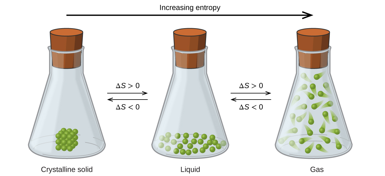
Figure\(\PageIndex{1}\): Entropy increases as a substance transitions from a solid to a liquid to a gas.

This is pretty easy to see because the particulate material becomes far more dispersed as it transitions from a solid to a liquid to a gas. Not only are the locations of the particles more dispersed in going from left to right, but they also gain more energy, and so each particle has more energy microstates available to it, thereby increasing the entropy of the system.

Temperature Changes

As the temperature increases the entropy increases due to the increased number of available states. This can be seen by the energy profile on the left part of figure 18.4.2 where the different kinetic energy states could be visualized as a type of microstate. That is, at lower temperatures most of the molecules are in lower energy states, but as the temperature increases more and more molecules enter higher energy states, and so the entropy of the system increases.

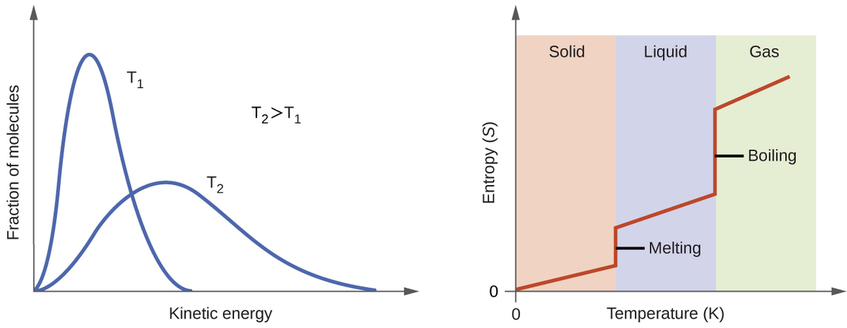
Figure\(\PageIndex{1}\): The left side shows an energy diagram for a gas and that at higher temperatures there are more states available. The right side shows how entropy is a function of both phase changes and temperature changes.

Mixing (Dissolution)

Typically, dissolution process involves an increase in entropy because a solid becomes more dispersed as it dissolves, but this is not always the case, because sometimes the solute introduces order into the solvent. For example, the dissolution of calcium hydroxide has a negative not positive entropy change

\[ Ca(OH)_2(s) \leftrightharpoons Ca(OH)_2(aq)\]

At first glance you would (incorrectly) think that the above equation represents an increase in entropy because Ca(OH)₂(aq) is more dispersed than Ca(OH)₂(s), which it is, but the water becomes more organized, and although water is not explicitly written in the above equation, it is the solvent of aqueous systems and the most common species. The water not only becomes oriented around the ions because of ion-dipole interactions, but in the case of many metal ions, form complex ions (see section 17.6). Hydroxide salts also have a common ion with the water and suppress its autodissociation (raising the pH) and so things can get real complex real quick. The important thing to note here is that the system is not just the solute, but the solute and the solvent, and sometimes a solute causes a decrease in the entropy of the solvent, and that effect is greater than the increase in entropy the solute itself undergoes. (In the case of calcium hydroxide, the solute (calcium hydroxide) did undergo an increase in entropy upon dissolution, but it induced a decrease in entropy of the solvent (water), so the net effect is a decrease in entropy.

Reactions that Change the Number of Particles

A reaction that increases the number of particles tends to increase the entropy because the greater the number of particles in a system, the greater the number of available microstates and thus the greater the entropy. But, if there is a phase change, that will have a larger effect. and so two gas particles becoming three solids would not have an increase in entropy.

Exercise \(\PageIndex{1}\)

Consider the following reactions of the nature 2A + B --> 2C. Indicate if they would have an increase or decrease in entropy, and give major reason why.

\[\begin{align} &(a.) \; \; 2C(s) + O_2(g) \rightarrow 2CO(g) \nonumber \\ &(b.) \; \; 2K(s) + Br_2(l) \rightarrow 2KBr(s) \nonumber \\ &(c.) \; \; 2H_2(g) + O_2(g) \rightarrow 2H_2O(g) \nonumber \end{align}\]

Answer

(a.) Increase, even though the total number of particles decrease, the number of gas phase increases.
(b.) Decrease, because liquid becomes solid, and there are less particles
(c.) Decrease, phase is the same, but number of particles decreases.

Size (Complexity) of Molecules

If you consider each bond as having different ways to vibrate, and possibly rotate, then the more bonds and the more complex a molecule, the more ways it can distribute energy, and so the more microstates it has. This results in an increase in entropy. So one would expect a complex molecule to have a higher entropy than a simple molecule.

Standard State Entropies

Because entropy is a state function the entropy of a reaction can be calculated through standard state molar entropies of formation the same way they can be calculated for enthalpies of reaction (review section 5.7.3, Standard Enthalpies of Formation).

Molar Entropy

The standard molar entropy is the entropy contained in one mole of a substance at standard state. The standard state values used in this text are P=1 bar (0.983 atm), T=298K and the concentration of a solute equal to a one molar solution. Note, the standard temperature may change between tables, so you should always look at the table to see the referenced temperature. In this class that will be 298K. Also, prior to 1982 the standard state pressure was 1 atm, and so older data tables may reference that pressure.

The molar entropy is analogous to the molar enthalpy of formation, and represents the energy change associated with the formation of a compound from its elements in their standard state, except that it is calculated for the change in entropy from absolute zero, when the value equaled 0.

For liquid water the equation would be

\[H_2(g) + \frac{1}{2}O_2 \rightarrow H_2O(l) \; \; \; S^o=69.91 \frac{J}{mol \cdot K}\]

Table of Molar Entropies

The following table has the molar entropies for select substances. Table T1 is a more comprehensive table, that can be found from the header of any LibreText chemistry page using the links Reference_Tables/Thermodynamics_Tables/T1:_Standard_Thermodynamic_Quantities.

Open Table

Substance	\(S^\circ_{298}\) (J mol−1 K−1)
carbon
C(s, graphite)	5.740
C(s, diamond)	2.38
CO(g)	197.7
CO2(g)	213.8
CH4(g)	186.3
C2H4(g)	219.5
C2H6(g)	229.5
CH3OH(l)	126.8
C2H5OH(l)	160.7
hydrogen
H2(g)	130.57
H(g)	114.6
H2O(g)	188.71
H2O(l)	69.91
HCI(g)	186.8
H2S(g)	205.7
oxygen
O2(g)	205.03

There are several important differences to note between the standard state molar entropy and standard state molar enthalpy of formation, as can be seen in figure 18.4.2.

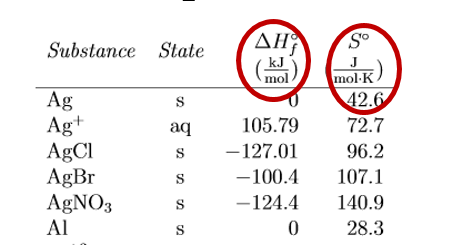
Figure\(\PageIndex{2}\): Comparison of standard entropies with standard molar enthalpies of formation.

Things to note in Figure \(\PageIndex{2}\):

1. \(\Delta H^o_f\) represents the change in forming something from its constituent elements at standard state while the molar entropy is not a \(\Delta \) and represents the actual value as compared to a value of zero at absolute zero. (see Molar Entropies: A Deeper Look)
2. Substances in the pure state (Ag(s) and Al(s)) have \(\Delta H^o_f\) =0 as it represents the change in forming them from themselves, but there is an entropy value, which is the difference in entropy of the pure substance at 298K in contrast to the value of oK (which equals 0).
3. There are never negative S^o values, but there can be negative \(\Delta H^o_f\) values.
4. The values of enthalpies are 1000 times larger, look at the units (kJ/mol, in contrast to J/mol-K).

deeper look at molar entropy as absolute value

Why does the standard molar entropy of formation for a pure substance not have a \(\Delta \), that is it is \(S^0_f\) and has a value for a pure element in it's standard state, while standard enthalpies (and Free Energies) are expressed with a \(Delta\), that is it is \(\Delta H^0_f\) or (\(\Delta G^0_f\)), and their values of formation equal zero for elements in their standard state.

Deeper Look

Energy values, as you know, are all relative, and must be defined on a scale that is completely arbitrary; there is no such thing as the absolute energy of a substance, so we can arbitrarily define the enthalpy or internal energy of an element in its most stable form at 298K and 1 atm pressure as zero. The same is not true of the entropy; since entropy is a measure of the “dilution” of thermal energy, it follows that the less thermal energy available to spread through a system (that is, the lower the temperature), the smaller will be its entropy. In other words, as the absolute temperature of a substance approaches zero, so does its entropy. This principle is the basis of the Third law of thermodynamics, which states that the entropy of a perfectly-ordered solid at 0 K is zero.

The absolute entropy of a substance at any temperature above 0 K must be determined by calculating the increments of heat q required to bring the substance from 0 K to the temperature of interest, and then summing the ratios q/T. Two kinds of experimental measurements are needed:

The enthalpies associated with any phase changes the substance may undergo within the temperature range of interest. Melting of a solid and vaporization of a liquid correspond to sizeable increases in the number of microstates available to accept thermal energy, so as these processes occur, energy will flow into a system, filling these new microstates to the extent required to maintain a constant temperature (the freezing or boiling point); these inflows of thermal energy correspond to the heats of fusion and vaporization. The entropy increase associated with melting, for example, is just ΔH_fusion/T_m. The heat capacity C of a phase expresses the quantity of heat required to change the temperature by a small amount ΔT , or more precisely, by an infinitesimal amount dT . Thus the entropy increase brought about by warming a substance over a range of temperatures that does not encompass a phase transition is given by the sum of the quantities C dT/T for each increment of temperature dT . This is of course just the integral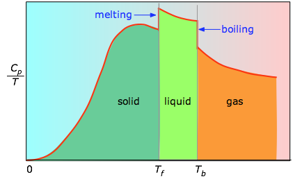

Figure \(\PageIndex{3}\): Heat capitity/temperature as a function of temperature

The area under each section of the plot represents the entropy change associated with heating the substance through an interval ΔT. To this must be added the enthalpies of melting, vaporization, and of any solid-solid phase changes. Values of C_p for temperatures near zero are not measured directly, but can be estimated from quantum theory.

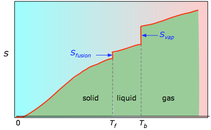
Figure \(\PageIndex{4}\): Molar entropy as a function of temperature

The cumulative areas from 0 K to any given temperature (taken from the experimental plot on the left) are then plotted as a function of T, and any phase-change entropies such as S_vap = H_vap / T_b are added to obtain the absolute entropy at temperature T. As shown in Figure \(\PageIndex{4}\) above, the entropy of a substance increases with temperature, and it does so for two reasons:

As the temperature rises, more microstates become accessible, allowing thermal energy to be more widely dispersed. This is reflected in the gradual increase of entropy with temperature. The molecules of solids, liquids, and gases have increasingly greater freedom to move around, facilitating the spreading and sharing of thermal energy. Phase changes are therefore accompanied by massive and discontinuous increase in the entropy.

\[ S_{0^o \rightarrow T^o} = \int _{o^o}^{T^o} \dfrac{C_p}{T} dt \]

Because the heat capacity is itself slightly temperature dependent, the most precise determinations of absolute entropies require that the functional dependence of C on T be used in the above integral in place of a constant C.

\[ S_{0^o \rightarrow T^o} = \int _{o^o}^{T^o} \dfrac{C_p(T)}{T} dt \]

When this is not known, one can take a series of heat capacity measurements over narrow temperature increments ΔT and measure the area under each section of the curve in Figure \(\PageIndex{3}\).

Entropy of Reaction

One can calculate the standard state entropy of reaction from standard molar entropies the same way one can calculate the enthalpy of reaction from the standard state molar enthalpies of formation (review section 5.7.4, Calculating Enthalpy of Reaction From Standard Enthalpies of Formation).

\[ΔS°=\sum nS^\circ_{298}(\ce{products})−\sum mS^\circ_{298}(\ce{reactants}) \label{\(\PageIndex{6}\)}\]

Where n and m represents stoichiometric coefficients of individual products and reactants in the balanced equation representing the process. For example, ΔS°_rxn for the following reaction at room temperature

\[m\ce{A}+n\ce{B}⟶x\ce{C}+y\ce{D} \label{\(\PageIndex{7}\)}\]

is computed as the following:

\[=[xS^\circ_{298}(\ce{C})+yS^\circ_{298}(\ce{D})]−[mS^\circ_{298}(\ce{A})+nS^\circ_{298}(\ce{B})] \label{\(\PageIndex{8}\)}\]

Table \(\PageIndex{2}\) lists some standard entropies at 298.15 K. You can find additional standard entropies in Tables T1 or T2.

Contributors and Attributions

Robert E. Belford (University of Arkansas Little Rock; Department of Chemistry). The breadth, depth and veracity of this work is the responsibility of Robert E. Belford, [e-mail]. You should contact him if you have any concerns. This material has both original contributions, and content built upon prior contributions of the LibreTexts Community and other resources, including but not limited to:

Some of this material was borrowed from OpenStax.,