
18.3: Entropy - A Microscopic Understanding
- Page ID
- 60790

\( \newcommand{\vecs}[1]{\overset { \scriptstyle \rightharpoonup} {\mathbf{#1}} } \)
\( \newcommand{\vecd}[1]{\overset{-\!-\!\rightharpoonup}{\vphantom{a}\smash {#1}}} \)
\( \newcommand{\id}{\mathrm{id}}\) \( \newcommand{\Span}{\mathrm{span}}\)
( \newcommand{\kernel}{\mathrm{null}\,}\) \( \newcommand{\range}{\mathrm{range}\,}\)
\( \newcommand{\RealPart}{\mathrm{Re}}\) \( \newcommand{\ImaginaryPart}{\mathrm{Im}}\)
\( \newcommand{\Argument}{\mathrm{Arg}}\) \( \newcommand{\norm}[1]{\| #1 \|}\)
\( \newcommand{\inner}[2]{\langle #1, #2 \rangle}\)
\( \newcommand{\Span}{\mathrm{span}}\)
\( \newcommand{\id}{\mathrm{id}}\)
\( \newcommand{\Span}{\mathrm{span}}\)
\( \newcommand{\kernel}{\mathrm{null}\,}\)
\( \newcommand{\range}{\mathrm{range}\,}\)
\( \newcommand{\RealPart}{\mathrm{Re}}\)
\( \newcommand{\ImaginaryPart}{\mathrm{Im}}\)
\( \newcommand{\Argument}{\mathrm{Arg}}\)
\( \newcommand{\norm}[1]{\| #1 \|}\)
\( \newcommand{\inner}[2]{\langle #1, #2 \rangle}\)
\( \newcommand{\Span}{\mathrm{span}}\) \( \newcommand{\AA}{\unicode[.8,0]{x212B}}\)
\( \newcommand{\vectorA}[1]{\vec{#1}} % arrow\)
\( \newcommand{\vectorAt}[1]{\vec{\text{#1}}} % arrow\)
\( \newcommand{\vectorB}[1]{\overset { \scriptstyle \rightharpoonup} {\mathbf{#1}} } \)
\( \newcommand{\vectorC}[1]{\textbf{#1}} \)
\( \newcommand{\vectorD}[1]{\overrightarrow{#1}} \)
\( \newcommand{\vectorDt}[1]{\overrightarrow{\text{#1}}} \)
\( \newcommand{\vectE}[1]{\overset{-\!-\!\rightharpoonup}{\vphantom{a}\smash{\mathbf {#1}}}} \)
\( \newcommand{\vecs}[1]{\overset { \scriptstyle \rightharpoonup} {\mathbf{#1}} } \)
\( \newcommand{\vecd}[1]{\overset{-\!-\!\rightharpoonup}{\vphantom{a}\smash {#1}}} \)
\(\newcommand{\avec}{\mathbf a}\) \(\newcommand{\bvec}{\mathbf b}\) \(\newcommand{\cvec}{\mathbf c}\) \(\newcommand{\dvec}{\mathbf d}\) \(\newcommand{\dtil}{\widetilde{\mathbf d}}\) \(\newcommand{\evec}{\mathbf e}\) \(\newcommand{\fvec}{\mathbf f}\) \(\newcommand{\nvec}{\mathbf n}\) \(\newcommand{\pvec}{\mathbf p}\) \(\newcommand{\qvec}{\mathbf q}\) \(\newcommand{\svec}{\mathbf s}\) \(\newcommand{\tvec}{\mathbf t}\) \(\newcommand{\uvec}{\mathbf u}\) \(\newcommand{\vvec}{\mathbf v}\) \(\newcommand{\wvec}{\mathbf w}\) \(\newcommand{\xvec}{\mathbf x}\) \(\newcommand{\yvec}{\mathbf y}\) \(\newcommand{\zvec}{\mathbf z}\) \(\newcommand{\rvec}{\mathbf r}\) \(\newcommand{\mvec}{\mathbf m}\) \(\newcommand{\zerovec}{\mathbf 0}\) \(\newcommand{\onevec}{\mathbf 1}\) \(\newcommand{\real}{\mathbb R}\) \(\newcommand{\twovec}[2]{\left[\begin{array}{r}#1 \\ #2 \end{array}\right]}\) \(\newcommand{\ctwovec}[2]{\left[\begin{array}{c}#1 \\ #2 \end{array}\right]}\) \(\newcommand{\threevec}[3]{\left[\begin{array}{r}#1 \\ #2 \\ #3 \end{array}\right]}\) \(\newcommand{\cthreevec}[3]{\left[\begin{array}{c}#1 \\ #2 \\ #3 \end{array}\right]}\) \(\newcommand{\fourvec}[4]{\left[\begin{array}{r}#1 \\ #2 \\ #3 \\ #4 \end{array}\right]}\) \(\newcommand{\cfourvec}[4]{\left[\begin{array}{c}#1 \\ #2 \\ #3 \\ #4 \end{array}\right]}\) \(\newcommand{\fivevec}[5]{\left[\begin{array}{r}#1 \\ #2 \\ #3 \\ #4 \\ #5 \\ \end{array}\right]}\) \(\newcommand{\cfivevec}[5]{\left[\begin{array}{c}#1 \\ #2 \\ #3 \\ #4 \\ #5 \\ \end{array}\right]}\) \(\newcommand{\mattwo}[4]{\left[\begin{array}{rr}#1 \amp #2 \\ #3 \amp #4 \\ \end{array}\right]}\) \(\newcommand{\laspan}[1]{\text{Span}\{#1\}}\) \(\newcommand{\bcal}{\cal B}\) \(\newcommand{\ccal}{\cal C}\) \(\newcommand{\scal}{\cal S}\) \(\newcommand{\wcal}{\cal W}\) \(\newcommand{\ecal}{\cal E}\) \(\newcommand{\coords}[2]{\left\{#1\right\}_{#2}}\) \(\newcommand{\gray}[1]{\color{gray}{#1}}\) \(\newcommand{\lgray}[1]{\color{lightgray}{#1}}\) \(\newcommand{\rank}{\operatorname{rank}}\) \(\newcommand{\row}{\text{Row}}\) \(\newcommand{\col}{\text{Col}}\) \(\renewcommand{\row}{\text{Row}}\) \(\newcommand{\nul}{\text{Nul}}\) \(\newcommand{\var}{\text{Var}}\) \(\newcommand{\corr}{\text{corr}}\) \(\newcommand{\len}[1]{\left|#1\right|}\) \(\newcommand{\bbar}{\overline{\bvec}}\) \(\newcommand{\bhat}{\widehat{\bvec}}\) \(\newcommand{\bperp}{\bvec^\perp}\) \(\newcommand{\xhat}{\widehat{\xvec}}\) \(\newcommand{\vhat}{\widehat{\vvec}}\) \(\newcommand{\uhat}{\widehat{\uvec}}\) \(\newcommand{\what}{\widehat{\wvec}}\) \(\newcommand{\Sighat}{\widehat{\Sigma}}\) \(\newcommand{\lt}{<}\) \(\newcommand{\gt}{>}\) \(\newcommand{\amp}{&}\) \(\definecolor{fillinmathshade}{gray}{0.9}\)Introduction
Ludwig Boltzmann developed a molecular-scale statistical model that related the entropy of a system to the number of microstates possible for the system. A microstate (\(\Omega\)) is a specific configuration of the locations and energies of the atoms or molecules that comprise a system like the following:
\[S=k \ln \Omega \\ or \\ S=k \ln W \label{Eq2}\]
Here k is the Boltzmann constant and has a value of 1.38 × 10⁻²³ J/K.
In general chemistry 1 we calculated ground state electron distributions where electrons resided in specific orbitals, which if we followed the Aufbau principle, the lowest energy state as the ground state. But if we added energy to the system, excited states could be obtained. Each of these states is a type of microstate. The ground state of helium would be 1S2 with both electrons being in the ground state. As we add energy to the system the temperature goes up, and the electrons can exist in various excited states. Entropy is related to the number of available states, and increases as the number of states increases. In reality we are discussing the ways energy and particles can be distributed in a system, and there are microstates related to the various translational, vibrational, and rotational modes energy can be distributed in a system
Entropy is also a state function, and so the energy difference between its final (Sf) and initial (Si) states is independent of the path:
\[ΔS=S_\ce{f}−S_\ce{i}=k \ln \Omega_\ce{f} − k \ln \Omega_\ce{i}=k \ln\dfrac{\Omega_\ce{f}}{\Omega_\ce{i}} \label{Eq2a}\]
For processes involving an increase in the number of microstates, \(\Omega_f > \Omega_i\), the entropy of the system increases, ΔS > 0. Conversely, processes that reduce the number of microstates, \(\Omega_f < \Omega_i\), yield a decrease in system entropy, ΔS < 0.
Consider the general case of a system composed of N particles distributed among n boxes. The number of microstates possible for such a system is nN. For example, distributing four particles among two boxes will result in 24 = 16 different microstates as illustrated in Figure \(\PageIndex{2}\). Microstates with equivalent particle arrangements (not considering individual particle identities) are grouped together and are called distributions. The probability that a system will exist with its components in a given distribution is proportional to the number of microstates within the distribution. Since entropy increases logarithmically with the number of microstates, the most probable distribution is therefore the one of greatest entropy.
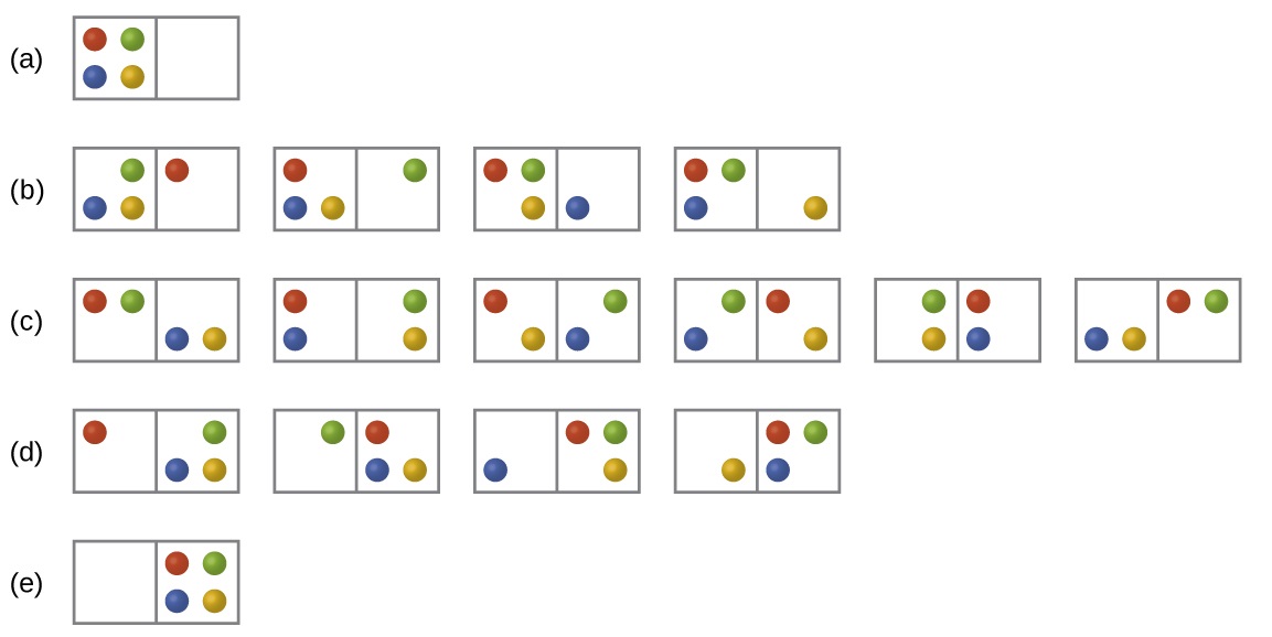
Figure \(\PageIndex{2}\): The sixteen microstates associated with placing four particles in two boxes are shown. The microstates are collected into five distributions—(a), (b), (c), (d), and (e)—based on the numbers of particles in each box.
The most probable distribution is therefore the one of greatest entropy.
For this system, the most probable configuration is one of the six microstates associated with distribution (c) where the particles are evenly distributed between the boxes, that is, a configuration of two particles in each box. The probability of finding the system in this configuration is
\[\dfrac{6}{16} = \dfrac{3}{8}\]
The least probable configuration of the system is one in which all four particles are in one box, corresponding to distributions (a) and (e), each with a probability of
\[\dfrac{1}{16}\]
The probability of finding all particles in only one box (either the left box or right box) is then
\[\left(\dfrac{1}{16}+\dfrac{1}{16}\right)=\dfrac{2}{16} = \dfrac{1}{8}\]
As you add more particles to the system, the number of possible microstates increases exponentially (2N). A macroscopic (laboratory-sized) system would typically consist of moles of particles (N ~ 1023), and the corresponding number of microstates would be staggeringly huge. Regardless of the number of particles in the system, however, the distributions in which roughly equal numbers of particles are found in each box are always the most probable configurations.
In section 18.1.3 we looked at the expansion of a gas into a vacuum. We took a statistical thermodynamic approach, the least probable configuration would be for all the particles to be in one bulb and none in the other (analogous to (a) and (s) of figure 18.3.2 (above) and this state would have the lowest entropy. The state with the highest entropy would have an equivalent number of particles in both bulbs, analogous to (c) above, and so going from the initial state to the final state would represent an increase in entropy.
Contributors and Attributions
Robert E. Belford (University of Arkansas Little Rock; Department of Chemistry). The breadth, depth and veracity of this work is the responsibility of Robert E. Belford, rebelford@ualr.edu. You should contact him if you have any concerns. This material has both original contributions, and content built upon prior contributions of the LibreTexts Community and other resources, including but not limited to:
Some of this material was borrowed from OpenStax.,