6.1: Reaction Rates

Learning Objectives

• Define chemical reaction rate
• Define and differentiate initial, instantaneous, and average rates as shown on a graph of concentration vs. time
• Relate the rates of change of any reactant and any product using the reaction stoichiometry

A rate measures how a quantity changes over time. Speed, for example, expresses the distance travelled per unit time, while wage represents the money earned per unit time. Similarly, the rate of a chemical reaction describes how quickly reactants are consumed or products are formed over time.

Reaction Rates

The rate of reaction is the change in the concentration of a reactant or product per unit time. Reaction rates are determined by measuring time-dependent changes in observable properties. For reactions involving gases, changes in volume or pressure can be measured. If a reaction involves a coloured substance, its rate can be monitored by changes in light absorption. For reactions with electrolytes, changes in solution conductivity can provide information about the rate.

The progress of a simple reaction (A → B) is shown in (Figure \(\PageIndex{1}\)). The beakers show snapshots of the reaction mixture at 10-second intervals, while the graph plots the number of molecules of reactant (A) and product (B) over time. Each point on the graph corresponds to one beaker in (Figure \(\PageIndex{1}\)). As the reaction proceeds, the concentration of A decreases and the concentration of B increases. The reaction rate is determined by the change in concentration of either species over a given time interval.

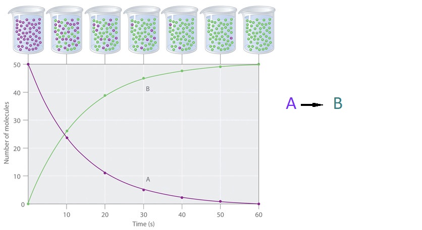
Figure \(\PageIndex{1}\): The Progress of a Simple Reaction (A → B). The mixture initially contains only A molecules (purple). Over time, the number of A molecules decreases and more B molecules (green) are formed. The graph shows the change in the number of A and B molecules in the reaction as a function of time over a 1 minute period.

\[\text { rate }=\frac{\Delta[\mathrm{B}]}{\Delta t}=-\frac{\Delta[\mathrm{A}]}{\Delta t} \nonumber\]

Square brackets indicate molar concentrations and the capital Greek delta (Δ) represents a change in value.  By convention, reaction rates are always expressed as positive numbers.  Since reactant concentrations decrease over time, the negative sign in -Δ[A]/Δt ensures the rate is reported as a positive quantity.  This equation shows that the reaction rate is equal to the negative rate of disappearance of A and is also equal to the rate of appearance of B.

Consider the decomposition of hydrogen peroxide (H₂O₂) in aqueous solution:

\[\ce{2H2O2}(aq)⟶\ce{2H2O}(l)+\ce{O2}(g) \nonumber \]

The rate of this reaction can be expressed in terms of the rate of change of [H₂O₂]:

\[\begin{align*}
\ce{rate\: of\: decomposition\: of\: H_2O_2}
&=\mathrm{−\dfrac{change\: in\: concentration\: of\: reactant}{time\: interval}}\\[4pt]
&=−\dfrac{[\ce{H2O2}]_{t_2}−[\ce{H2O2}]_{t_1}}{t_2−t_1}\\[4pt]
&=−\dfrac{Δ[\ce{H2O2}]}{Δt}
\end{align*} \nonumber \]

where:

•  \([\ce{H2O2}]_{t_1}\) is the molar concentration of hydrogen peroxide at initial time t₁
• \([\ce{H2O2}]_{t_2}\) represents the molar concentration of hydrogen peroxide at a later time t₂
• \(Δ\left\lbrack H_2O_2\right\rbrack\) represents the change in molar concentration of hydrogen peroxide during the time interval Δt (that is, t₂ − t₁)

Since the reactant concentration decreases as the reaction proceeds, Δ[H₂O₂] is a negative quantity.  The negative sign in the equation ensures the reaction rate is expressed as a positive quantity, consistent with standard convention. Figure \(\PageIndex{2}\) provides an example of data collected during the decomposition of H₂O₂.

Figure \(\PageIndex{2}\): The rate of decomposition of H₂O₂ in an aqueous solution decreases as the concentration of H₂O₂ decreases.

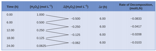
To obtain data for this decomposition, the concentration of hydrogen peroxide was measured every 6 hours over a 24-hour period at a constant temperature of 40 °C. Reaction rates were calculated for each time interval by dividing the change in concentration by the corresponding time increment, as shown for the first 6-hour period:

\[\dfrac{−Δ[\ce{H2O2}]}{Δt}=\mathrm{\dfrac{−(0.500\: mol/L−1.000\: mol/L)}{(6.00\: h−0.00\: h)}=0.0833\: mol\:L^{−1}\:h^{−1}} \nonumber \]

As the reaction proceeds, the rate decreases over time. For the last 6-hour period, the reaction rate is:

\[\dfrac{−Δ[\ce{H2O2}]}{Δt}=\mathrm{\dfrac{−(0.0625\:mol/L−0.125\:mol/L)}{(24.00\:h−18.00\:h)}=0.0104\:mol\:L^{−1}\:h^{−1}} \nonumber \]

These values show that the rate of reaction decreases with time. 

Since reaction rates vary over time, it is important to specify which rate is being discussed:

•     Average rate: the change in concentration of a reactant or product over a finite time interval.
•     Instantaneous rate: the rate of reaction at a specific moment in time.
•     Initial rate: the instantaneous rate at t=0, when the reaction first begins.

To illustrate this concept, consider a car slowing down as it approaches a stop sign. The initial rate of the car (analogous to the reaction’s initial rate) is the speedometer reading when the brakes are first applied. A few seconds later, the instantaneous rate (analogous to the reaction rate at a given time) is the speedometer reading at that moment. The average rate over the entire deceleration period is the total distance travelled divided by the total time required to stop. Like a decelerating car, a chemical reaction’s average rate falls between its initial and final rates.

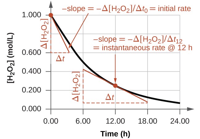
The instantaneous rate of a reaction can be determined in two ways. If experimental conditions allow for the measurement of concentration changes over very short time intervals, then average rates, as previously described, can approximate instantaneous rates. Alternatively, as shown in the Figure \(\PageIndex{3}\), calculus can be used to determine the instantaneous rate of change at any given time by finding slope of a tangent line at that point.

Figure \(\PageIndex{3}\): This graph shows a plot of concentration versus time for a 1.000 M solution of H₂O₂. The rate at any instant is equal to the negative of the slope of a line tangent to this curve at that time. Tangents are shown at t = 0 h (“initial rate”) and at t = 12 h (“instantaneous rate” at that particular time).

Reaction Rates in Analysis: Test Strips for Urinalysis

Physicians often use disposable test strips to measure the amounts of various substances in a patient’s urine (Figure \(\PageIndex{4}\)). These strips contain chemical reactants embedded in small pads, which undergo colour changes upon exposure to specific substances at sufficient concentrations. The usage instructions for test strips often stress that proper read time is critical for optimal results. This emphasis on read time suggests that kinetic aspects of the chemical reactions occurring on the test strip are important considerations.

The test for urinary glucose relies on a two-step reaction:

\[\ce{C6H12O6 + O2}\underset{\large\textrm{catalyst}}{\xrightarrow{\hspace{45px}}}\ce{C6H10O6 + H2O2} \nonumber \]

\[\ce{2H2O2 + 2I-}\underset{\large\textrm{catalyst}}{\xrightarrow{\hspace{45px}}}\ce{I2 + 2H2O + O2} \nonumber \]

In the first reaction, glucose is oxidized to produce glucolactone and hydrogen peroxide. The hydrogen peroxide then oxidizes colourless iodide ions into brown iodine, which is visually detected. Some strips include additional reagents that enhance the colour contrast for easier interpretation.

These reactions are slow, but enzymes embedded in the test strip significantly speed up the process—a phenomenon known as catalysis, which will be discussed later in this chapter. A typical glucose test strip takes about 30 seconds for the colour to fully develop. Reading the strip too soon may lead to a false negative, underestimating the glucose concentration. Conversely, waiting too long may result in a false positive, as uncatalyzed oxidation by other substances in urine gradually darkens the test area.

Figure \(\PageIndex{4}\): Test strips are commonly used to detect the presence of specific substances in a person’s urine. Many test strips have several pads containing various reagents to permit the detection of multiple substances on a single strip. (credit: Iqbal Osman).

Relative Rates of Reaction

The rate of a reaction can be expressed in terms of the change in concentration of any reactant or product. The relative rates of reactant consumption and product formation are determined by the reaction’s stoichiometry.

For a balanced reaction equation:

\[\ce{aA} + {bB} ⟶\ce{cC} + \ce{dD} \nonumber \]

The reaction rate can be expressed using the stoichiometric coefficients:
\[\text { rate }=-\left(\frac{1}{\mathrm{a}}\right)\left(\frac{\Delta \mathrm{[A]}}{\Delta t}\right)=-\left(\frac{1}{\mathrm{~b}}\right)\left(\frac{\Delta \mathrm{[B]}}{\Delta t}\right) = \left(\frac{1}{\mathrm{~c}}\right)\left(\frac{\Delta \mathrm{[C]}}{\Delta t}\right) = \left(\frac{1}{\mathrm{~d}}\right)\left(\frac{\Delta \mathrm{[D]}}{\Delta t}\right)\]

Since reaction rates are conventionally positive, the rate of disappearance of reactants is given a negative sign to reflect their decreasing concentration.

Consider the reaction:

\[\ce{2NH3}(g)⟶\ce{N2}(g)+\ce{3H2}(g) \nonumber \]

The relative rates of reactant consumption and product formation follow from the stoichiometric coefficients. The relationship between the rates of nitrogen production and ammonia consumption is:

\[−\dfrac{1}{2}\dfrac{Δ[\ce{NH3}]}{Δt}=\dfrac{Δ[\ce{N2}]}{Δt} \nonumber \]

Note that a negative sign has been added to account for the opposite signs of the two amount changes (the reactant amount is decreasing while the product amount is increasing). 

Similarly, since three moles of H₂ form for every one mole of N₂ produced, the rate of H₂ formation is three times the rate of N₂ formation:

\[\dfrac{1}{3}\dfrac{Δ[\ce{H2}]}{Δt}=\dfrac{Δ[\ce{N2}]}{Δt} \nonumber \]

Figure \(\PageIndex{5}\) illustrates the concentration changes over time for the decomposition of ammonia at 1100 °C. The slopes of the tangents drawn at t = 500 seconds confirm that the instantaneous rates of change in the concentrations of the reactants and products are related by their stoichiometric factors. For example, the rate of hydrogen production is observed to be approximately three times greater than the rate of nitrogen production:

\[\dfrac{2.91×10^{−6}\:M/\ce s}{9.70×10^{−7}\:M/\ce s}≈3 \nonumber \]

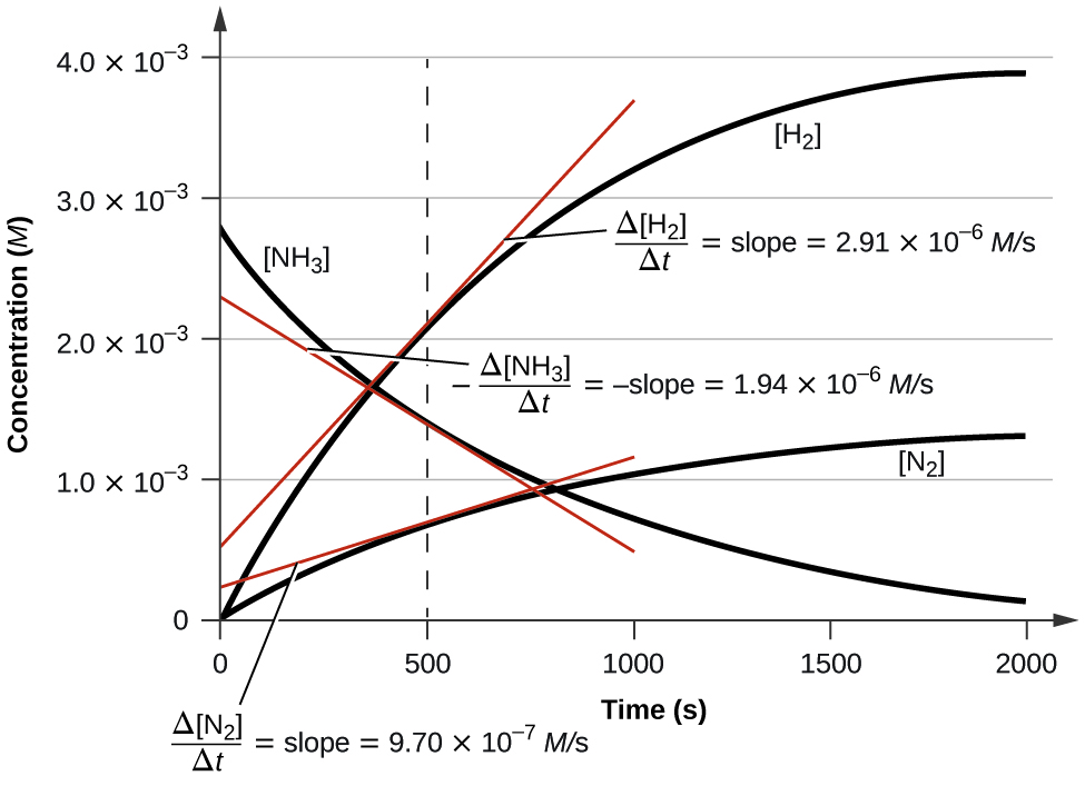
Figure \(\PageIndex{5}\): This graph shows the changes in concentrations of the reactants and products during the reaction \(\ce{2NH3⟶N2 + 3H2}\). The rates of change of the three concentrations are related by their stoichiometric factors, as shown by the different slopes of the tangents at t = 500 s.

Example \(\PageIndex{1}\)

Consider the conversion of dinitrogen tetroxide, N₂O₄ (g) to nitrogen dioxide, NO₂ (g):

\[ \mathrm{N}_2 \mathrm{O}_4(\mathrm{~g}) \ ⟶ 2 \mathrm{NO}_2(\mathrm{~g}) \nonumber\]

Write the rate expression for the reaction in terms of disappearance of the reactants and appearance of the products.

Solution

For every one mole of reactant that disappears, two moles of product are formed. The rate of disappearance of N₂O₄ must be must be half of the rate of appearance of NO₂. The rate of reaction therefore may be expressed as:

\[\text { rate } = −\dfrac{\mathrm{Δ[\:N_2O_4]}}{Δt}=\dfrac{1}{2}\dfrac{\mathrm{Δ[\:NO_2]}}{Δt} \nonumber \]

Example \(\PageIndex{2}\): Expressions for Relative Reaction Rates

The first step in the production of nitric acid is the combustion of ammonia:

\[\ce{4NH3}(g)+\ce{5O2}(g)⟶\ce{4NO}(g)+\ce{6H2O}(g) \nonumber \]

Write the equations that relate the rates of consumption of the reactants and the rates of formation of the products.

Solution

Considering the stoichiometry of this homogeneous reaction, the rates for the consumption of reactants and formation of products are:

\[−\dfrac{1}{4}\dfrac{Δ[\ce{NH3}]}{Δt}=−\dfrac{1}{5}\dfrac{Δ[\ce{O2}]}{Δt}=\dfrac{1}{4}\dfrac{Δ[\ce{NO}]}{Δt}=\dfrac{1}{6}\dfrac{Δ[\ce{H2O}]}{Δt} \nonumber \]

Exercise \(\PageIndex{1}\)

The rate of formation of Br₂ is 6.0 × 10⁻⁶ mol/L/s in a reaction described by the following net ionic equation:

\[\ce{5Br- + BrO3- + 6H+ ⟶ 3Br2 + 3H2O} \nonumber \]

Write the equations that relate the rates of consumption of the reactants and the rates of formation of the products.

Answer

\[−\dfrac{1}{5}\dfrac{Δ[\ce{Br-}]}{Δt}=−\dfrac{Δ[\ce{BrO3-}]}{Δt}=−\dfrac{1}{6}\dfrac{Δ[\ce{H+}]}{Δt}=\dfrac{1}{3}\dfrac{Δ[\ce{Br2}]}{Δt}=\dfrac{1}{3}\dfrac{Δ[\ce{H2O}]}{Δt} \nonumber \]

Example \(\PageIndex{3}\): Reaction Rate Expressions for Decomposition of H₂O₂

The graph in Figure \(\PageIndex{3}\) shows the rate of the decomposition of H₂O₂ over time:

\[\ce{2H2O2 ⟶ 2H2O + O2} \nonumber \]

Based on these data, the instantaneous rate of decomposition of H₂O₂ at t = 11.1 h is determined to be 3.20 × 10⁻² M/h, that is:

\[−\dfrac{Δ[\ce{H2O2}]}{Δt}=\mathrm{3.20×10^{−2}\:M\:h^{−1}} \nonumber \]

What are the instantaneous rates of production of H₂O and O₂ at 11.1 h?

Solution

From the stoichiometry of the reaction, we know:

\[−\dfrac{1}{2}\dfrac{Δ[\ce{H2O2}]}{Δt}=\dfrac{1}{2}\dfrac{Δ[\ce{H2O}]}{Δt}=\dfrac{Δ[\ce{O2}]}{Δt} \nonumber \]

For O₂:

\[\mathrm{\dfrac{1}{2}×3.20×10^{−2}\:M\:h^{−1}}=\dfrac{Δ[\ce{O2}]}{Δt} \nonumber \]

\[\dfrac{Δ[\ce{O2}]}{Δt}=\mathrm{1.60×10^{−2}\:M\:h^{−1}} \nonumber \]

For H₂O:

\[−\dfrac{1}{2}\dfrac{Δ[\ce{H2O2}]}{Δt}=\dfrac{1}{2}\dfrac{Δ[\ce{H2O}]}{Δt} \nonumber \]

\[\dfrac{Δ[\ce{H2O}]}{Δt}=\mathrm{3.2×10^{−2}\:M\:h^{−1}} \nonumber \]

Exercise \(\PageIndex{2}\)

If the rate of decomposition of ammonia, NH₃, at 1150 K is 2.10 × 10⁻⁶ M/s, what are the rates of production of nitrogen and hydrogen?

\[\ce{2NH3}(g)⟶\ce{N2}(g)+\ce{3H2}(g) \nonumber \]

Answer

1.05 × 10⁻⁶ M/s, N₂ and 3.15 × 10⁻⁶ M/s, H₂.

Summary

The rate of a reaction can be expressed as the decrease in reactant concentration or the increase in product concentration per unit time. The relationships between different rate expressions are determined by the stoichiometric coefficients of the balanced equation.

The average rate is calculated as the change in concentration over a given time interval. The instantaneous rate refers to the rate at a specific moment in time and is determined by the slope of a tangent line on a concentration vs. time graph. The initial rate is the instantaneous rate at t=0, when the reaction begins.