8: Formation Constants and Complex Ions

Learning Objectives

Goals: 

• Understand what coordination complexes are
• Describe the formation of a coordination complex in terms of Lewis Acid-Base Theory
• Understand the method of continuous variations
• Calculate K_f from from spectroscpopic data

By the end of this lab, students should be able to:

• Design an experiment using Job Plot (the method of successive variations)
• Predict the formula for a complex ion using a Jobs plot
• Use a Job plot to calculate K_f.

Prior knowledge:

• Lewis Acids and Bases (section 16.7)
• Equilibrium Involving Complex Ions (section 17.6)
• Equilibrium Chemistry (section 15.4)
• Mechanisms (section 14.6)

Overview

An acid/base pH titration is an analytical technique where the pH is measured as a function of the amount of titrant (strong acid or base) that is added to the analyte (base or acid). The analyte is initially the excess reagent until the amount of titrant required to exactly neutralize the analyte has been added (equivalence point), at which point they are in stoichiometric proportions. Upon further addition of titrant the analyte becomes the limiting reagent and the pH is dictated by the excess titrant. In a pH titration the pH is changing for two reasons, (1) neutralization and (2) dilution. In a Job's plot the total volume is kept constant and so the reactant and product concentrations are not influenced by dilution. Unlike a titration where you continually add one reactant to another and measure the effect, in a Job's plot each measurement is a unique solution where the mole fraction of reactants are varied.  So if a Job's plot had 20 measurements you would need to make 20 different solutions, where each solution represented different mole fraction ratios. Another name for the Job's Plot is the method of continuous variations and in this lab the Job's plot technique will be be applied to the formation of a coordination complex ion. 

Coordination Complexes

Many metal ions have vacant d orbitals that allow them to function as Lewis Acids (electron acceptors) that can react with molecules (or ions) with lone pairs of electrons, the Lewis bases (electron donors). These reactions can result in the formation of a coordination complex (sections 16.7: & 17.6), which is often highly colored. In this type of reaction the Lewis base is called the Ligand (L) and may be neutral (NH₃, H₂O,...) or charged (Cl^-, NO₂^-, ...).  The sum of the charges of the metal cation and all the ligands bonded to it gives the charge of the coordination complex, which may result in a neutral, cationic (positive) or anionic (negative) complex.  Charged coordination complexes are known as complex ions and are often soluble and highly colored. A complex ion consists of a central metal atom and a specific number of ligands covalently bonded to it, which determines its chemical formula. Water is a typical Lewis base and common aqueous metal ions like Fe⁺²,  Fe⁺³,  Cu⁺² and Al⁺³ ​form complex ions with water, that is, they form covalent bonds with the water, where both electrons come from the water. 

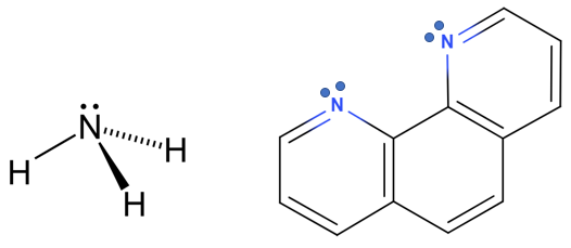
In the last experiment (Exp 7) you noted the entropy decreased even though it seems logical that dissolving a solid would result in increased entropy (which it often does). One reason for this is the formation of complex ions around cations, where the decrease in entropy of the solvent is greater than the increase in entropy of the solute. For example, the six water molecules of figure \(\PageIndex{1}\), are no longer free moving entities and thus the formation of the complex ion resuted in a decrease in entropy for the solvent, while the metal ion had an increase in entropy as it went from the solid to aqueous phase. Coordination complexes will be studied in more detail when we get to chapter 20 and for this lab it suffices to know that a complex ion can form from the Lewis Acid-Base reaction between a metal cation and a ligand (sections 16.7: & 17.6). 

Figure \(\PageIndex{1}\): Ball and stick and "pseudo" Lewis dot structure of hexaaqua iron (III) . Nomenclature of these will be covered in section 20.3 and what needs to be noted here is that the water is functioning as a ligand, and forms dative coordinate covalent bonds to the metal ion.  In the Lewis dot structure the two electrons of the lone pair from the water are shown in red and the arrow indicates that both electrons of the covalent bond come from the water, (which is acting as a Lewis base, an electron donor).

A ligand may be monatomic (Cl^-) or polyatomic (NH₄⁺). For polyatomic ligands the donor atom of the ligand is the atom that has the lone pair of electrons that form the coordinate covalent bond with the metal ion (oxygen is the donor atom of water in figure \(\PageIndex{1}\)). A polyatomic ligand may have more than one donor atom and thus form more than one coordinate covalent bond.  In figure \(\PageIndex{2}\) there are two ligands where nitrogen functions as the donor atoms.  A ligand with one donor atom is classified as a monodentate ligand, a ligand with two donor atoms is a bidentate ligand, and there are common polydentate ligands with up to 6 donor atoms. 

Figure \(\PageIndex{2}\): Two Ligands, ammonia (monodentate) and phenanthroline (bidentate)

The resulting coordination complex has a specific number of coordinate covalent bonds, which is the coordination number of the complex.  Figure \(\PageIndex{3}\) shows generic coordination complexes with various numbers of monodentate ligands and one bidentate ligand. The coordination number is only equal to the number of ligands if the ligands are monodentate, and in the case of the bidentate ligand with a formula ML₃ the coordination number (CN) is 6. Typical coordination numbers vary from 2 to 6 and the complexes have geometries similar to the VSEPR geometries we learned about in the first semester of the class.

Figure \(\PageIndex{3}\): Formula and coordination number for different coordination complexes. Note the complex ion on the right involves a bidentate ligand where oxygen is the donor atom and the formula ML₃ results in a coordination number of 6.

In this experiment we will be creating a highly colored complex ion between ferrous iron (Fe⁺²) and a neutral bidentate ligand (figure \(\PageIndex{2}\)).  We will then determine the formula for the complex ion and its formation constant. The generic equation for the formation of a complex with "b" ligands has the following form and formation constant (K_F).

\[M + bL \rightleftharpoons ML_b \;\; \;\;\left ( K_f=\frac{[ML_b]}{[M][L]^b} \right )\]

We will use absorbance spectroscopy and make measurements at a wavelength where the metal and the ligand are both colorless, but the complex ML_b is highly colored, and thus monitor the formation of the complex by the intensity of its color. The technique we will used is called the Job's Plot, or the method of continuous variations.

Job's Plot

A Job's plot is also know as the method of continous variations, where you measure the concentration of the product after varying the mole fractions of the reactants, and then plot the concentration of product as the dependent variable, with the mole fractions as the independent variable.  Since there are only two species there are two scales on the x axis, one for the mole fraction ligand and the other for the mole fraction of the metal, and they are related by the equation  X_M + X_L = 1.  

 

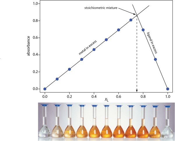
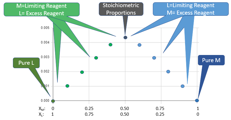Figure \(\PageIndex{4}\): Regions of Job Plot. Note, the scale on the X-axis shows the mole fractions of metal (X_M) and Ligand (X_L) and since these are related to each other (X_M + X_L=1), with the fraction varying from pure ligand on the left to pure metal on the right.  The peak represents when they are mixed in stoichiometric proportions.  (Belford)

The peak of jobs plot identifies the ratio of ligand to metal at stoichiometric proportions and thus allows one to determine the formula of the coordination complex. One can also look at the ratios of the slopes to in the regions away from stoichiometric proportions to determine the formula and you will be asked to devise this technique in your report.  When doing so it is important to realize that you are not measuring the reactant concentrations but the product concentration, which is plotted as a function of the reactant mole fraction.

Comparing Job's Plot to a Titration

Both titrations and Job's plots start with a pure reactant and then measure some effect from adding a second substance that reacts with the first. In an acid base reaction this is the hydronioum ion concentration (pH).  It should be emphasized that acid-base titrations are only one type of titration, and other types of titrations like redox titrations are common.  In a titration there is only one solution and you make measurements as you successively add the titrant. In the Job's plot each measurement is a different solution. In the titration the concentration of the initial reactant (analyte) is being reduced by two processes, reaction with the titrant and dilution, as the total volume of the solution increases as you add titrant. In the Job's plot you keep the total volume constant while varying the proportions of the different reagents mixed. In both titrations and Job's plots you need a way to measure the progress of the reaction.  In pH titrations this can be down with an indicator or pH meter. In a Job's plot this is often done with spectroscopy because the complexes are often highly colored, while the metal solutions and ligands are often colorless.

Absorbance Spectroscopy

In the first semester we learned that light can be absorbed by atoms if the energy of the light (E = h\(\nu\), h=Planck's constant) was equal to the energy gap between two electronic oribtals (section 6.3), and this resulted in a line spectra that could be used to identify an isolated gas phase atom. UV-Vis absorbance spectroscopy utilizes a similar technique in that light is transmitted through a solution and light of a frequency associated with electronic transitions of molecules within the solution are absorbed, with a subsequent reduction in the intensity of the transmitted light at that frequency as it exits the solution.  This technique can be used for both qualitative and quantitative analysis. A spectrum is a plot of the absorbance as a function of the wavelength of light and can be used to identify a molecule. If you measure the absorbance at a constant wavelength as a function of the solute concentration you get a linear "Beer's Law" plot that can be used in quantitative analysis. Figure \(\PageIndex{5}\) shows the absorbance spectrum for chlorophyll a and b on the left, and a Beer's law plot for chlorophyll a that was taken at 654 nm.

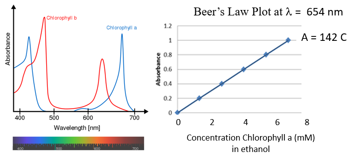Figure \(\PageIndex{5}\): Vis spectra of chlorophyll (left, Wikimedia Commons) and a plot of the absorbance as a function of concentration (right) in ethanol, note the spectrum  shows that chlorophyll absorb blue and red light and so it is green. (CC-BY: Belford)

We do not directly measure absorbance, instead we measure the reduction in the intensity of light as it passes through a sample, which is held in a special transparent container of known pathlength called the cuvette (figure \(\PageIndex{6}\)). In the first semester we learned that light has wave-particle duality (section 6.2) and the intensity of light is the number of moles of photons (n) times the energy of each photon (I=nh\(\nu\)), where h is Planck's constant. In figure \(\PageIndex{6}\), I_o represents the light entering the cuvette (the path length is zero) and I_t represents the light transmitted.  If some of the molecules absorb photons of a specific wavelength (as electrons are excited to higher energy states) the number of photons at that wavelength exiting the cuvette are less than entering, and so I_t < I_o at that wavelength.  The absorbance values (A) plotted in figure \(\PageIndex{5}\) are calculated from measurements of the change in intensity as the light travels through the cuvette. A spectrum results if these measurements are plotted across different wavelengths (left), and a Beer's plot results if they are plotted as a function of concentration at constant wavelength (right).

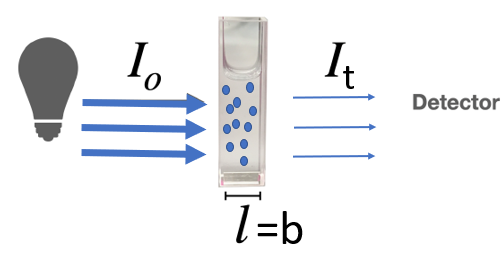Figure \(\PageIndex{6}\): Light of intensity I₀ enters cuvette of path length b that is of a frequency that is absorbed by the blue molecules and so the light transmitted (I_t) has a reduced intensity. (CC-BY; Kathryn Haas, modified by Belford)

There are three factors that influence the number of photons absorbed as light travels through a sample;

1. Path length (the longer the path length the greater the number photons absorbed).
2. Concentration of absorbing molecules (typically solute molecules, the more concentrated the more photons absorbed)
3. Intensity of the light itself (more photons are absorbed if you shine a bright light on a sample than a dim light). 

This latter effect is mathematically the same as first order kinetics where the rate of change in the concentration of a reactant was proportional the reactant's concentration (\(\frac{\Delta [A]}{\Delta t}=-k[A]\)). Here it is the rate of change in intensity of light that is proportional to the intensity itself (\(\frac{\Delta I}{\Delta x}=-kI\)), and it is related to the distance traveled (path length \(\Delta x = b\)) and not the time, as in kinetics.  As in the kinetics chapter, this requires calculus to solve and results in a logarithmic relationship that for historical reasons is written in log base 10. The general relationship is 

\[\Delta I =-kcI\Delta x\] where k is a proportionality constant, \(\Delta\)x is the change in path length, c is the concentration and I is the light intensity.

Integrating this from the calculus (see "Deeper Dive") gives us the relationship

\[log \frac{I_0}{I_t}=\epsilon bc\]

Absorbance (A) is defined as

\[A=log \frac{I_0}{I_t}\]

 and this results in Beer's Law, which is the relationship you need to use in this lab.

\[A=\epsilon bc\]

where,
A=absorbance
\(\epsilon\) = the extinction coefficient or the molar absorptivity constant with typical units of M^-1cm^-1.
b = path length
c = concentration of absorbing molecules

Students need to know Beer's Law but are not required to derive it. You will use a spectrometer that will read the absorbance for solutions of various concentrations. 

Deeper Dive

Note, Beer's law comes from the calculus and the absorbance (A) is related to the log of the intensity change. This logarithmic relationship is similar to first order kinetics where the rate of change in concentration of a reactant was proportional to the concentration of the reactant, but here it is the rate of change in intensity of light is proportional to the intensity of light.

\[dI = -kcIdx \\ \; \\ \frac{dI}{I}=-kcdx \\ \; \\ \int_{I_o}^{I_t}\frac{dI}{I}=-\int_{0}^{b}kcdx
\\ \; \\ lnI_t-ln_o = ln(\frac{I_t}{I_0})=-kcb \\ \; \\ ln(\frac{I_o}{I_t})=kcb\]

So after converting to log base 10 (which is done for historical reasons) we get

\[A=log \frac{I_0}{I_t}=\epsilon bc\]

Where A is the unitless absrobance, I_o is the intensity of light entering the sample, I_t is the intensity of light transmitted out of the sample, b is the path length, c is the concentration of the molecule absorbing the light and \(\epsilon\) is the extinction coefficient and has the units of concentration^-1 length^-1. The extinction coefficient is often a very large number which allows one to measure very small concentrations of solute, and it is a property of the molecule, but is influenced by the solvent.

 

Limitations of Beer's Law

Beer's Law is linear over a small range of absorbances and you can not believe all readings a spectrometer gives you.  The rule of thumb that we will use in this lab applies only to the spectrometers we use, and that is that we can only trust values between A= 0.05 and A=1.0.  There are two types of reasons for nonlinearity, chemical and instrumental.

Instrumental deviations from linearity typically relate to the sensitivity of the detection system. At low absorbances the limit of detectivity may be reached and the detector simply can't "see" the light.  At high absorbances the detector can get saturated and simply can't see anymore light.  Chemical reasons for nonlinearity typically involve solutes aggregating at high concentrations, which changes the spectra. It should also be noted that the solvent can affect the spectra of solute molecules.

If a solution is too concentrated (A>1) you simply need to dilute it until it is in the correct range.  In this class we are using the range of 0.05 to 1.0 as a "rule of thumb", but you can take a more concentrated solution, dilute it several times, and see if you still have a linear function.  The sensitivity of the photo detectors is not uniform across all wavelengths and you may find that at some wavelengths the system works at absorbances greater than 1, while at others it does not.  To be safe, use this range.

One of the advantages of spectroscopy is that it allows one to measure dilute solutions, and it is always easy to dilute a concentrated solution (simply add solvent), and so if the absorbance is greater than one, all you have to do is dilute the solution.  

The experiment:

During class you are to do the first Google Doc (Part 1) that was released as a group assignment.  Each student should then work up the data on a second Google Doc (Part 2) that is an individual assignment.  Students are welcome to collaborate on the individual assignments, but each student needs to submit their own work for grading in the Google Classroom.

1. Fill 50 mL burette with 0.005 M ferous iron.
2. Fill 50 mL burette with 0.005 M unkown ligand
3. Label thirteen 50 mL beakers with the mole fractions of iron as in the data acquisition table of your Google Doc (step 4) 
4. Wait at least 20 minutes for the reaction to complete
5. Choose wavelength for absorbance measurments
   1. Zero out the spectrometer with a blank solution of water
   2. Take a spectra of the darkest solution
   3. Choose a wavelength where the darkest solution approaches 1
   4. Write this wavelength down on the Google Doc (step 4., be sure to include units)
6. Record the absorbance of each solution in Google Doc (step 4) at the wavelength chosen in step 5.4
7. Double check that the reaction is over by checking the solutions that represent stoichiometric proportions of the hypothetical complexes to see if the absorbance has increased. Once all solutions maintain a constant value you can work up the data.

Figure \(\PageIndex{7}\): Solutions and their respective absorbances, note these values are ploted against mole fraction of ligand and in this experiment we will plot our against the mole fraction metal.  This reaction also goes to completion (image credit: David Harvey)

 

Data Workup:

 

Inserting Charts Into Google Docs

You need to make your Job's plot in Google Sheets and then paste it into your Google Doc.  To paste a Google Chart from a Google Sheet to a Google Doc you should follow the following steps.

1. Click the mouse on the Google Doc where you want the sheet (inside the table cell for this assignment)
2. Click Insert>Chart>From Sheets (left image of figure \(\PageIndex{6}\))
3. Type the name of sheet you are looking for, or part of its name (middle image of figure \(\PageIndex{6}\)), click on it and choose Select
4. Choose the chart you want to insert, (right image of figure \(\PageIndex{6}\)) click on it and choose Import

Figure \(\PageIndex{8}\): Screen capture of procedures for inserting a chart from a Google Sheet into a Google Doc

 

Calculating C_REAL

We know that A=\(\epsilon bc\) and so we can take the two state approach to relate the two variables at two different states as we did in kinetics (section 13.3.3.2) and with gas laws (section 10.2.4).  It should be noted the C represents the complex ion concentration ([ML_b]⁺² for a complex with b ligands.

\[\frac{A_1}{A_2} =\frac{\epsilon bC_1}{\epsilon bC_2} \\ \; \\ so \\ \; \\ \frac{A_1}{A_2} =\frac{C_1}{C_2}\]

Where state one is the hypothetical state if the reaction went to completion (100% yield, ie., A_MAX and C_MAX) and state 2 is the real state representing an equilibrium between reactants and products ( A_REAL and C_REAL)).  We can calculate C_MAX from the complete consumption of the limiting reagent (theoretical yield), measure A_REAL and determine A_MAX by extrapolating the absorbance in the excess ligand region to the value at stoichiometric proportions (see note at bottom of page).

Figure \(\PageIndex{9}\): Generic Job plot where X values indicate real data and the line is the extrapolation from regions where one reagent was in excess. 

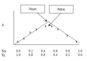
So \[C_{REAL}=C_{MAX}\frac{A_{REAL}}{A_{MAX}}\]

Calculating K_f

Figure \(\PageIndex{9}\) represents the formation of the complex ML because the peak is when the mole fraction of M and L are both 0.5.  If we look at the complex MLb where "b" is the number of ligands we have three possible equilbrium constants and the following generic RICE diagram.

\[M + L \rightleftharpoons ML \;\;\left ( K_f=\frac{[ML]}{[M][L]} \right ) \\ \; \\ M + 2L \rightleftharpoons ML_2 \;\; \;\;\left ( K_f=\frac{[ML_2]}{[M][L]^2} \right ) \\ \;\\ M + 3L \rightleftharpoons ML_3 \;\;\;\;\left ( K_f=\frac{[ML_3]}{[M][L]^3} \right )\]

Reactants	M	+	bL	⇌	MLb
Initial	[M]Initial		[L]Initial		0
Change	-x		-bx		+x
Equilibrium	[M]Eq=[M]Initial-x		[L]Eq=[L]Initial-bx		[MLb]Eq=x

noting C_REAL is ML_b because it is the complex ion that is absorbing the light.  So we know know the extent of reaction (x), and can solve for the eqiulibrium concentration of all species using the K_f expression appropriate to the complex ion being formed (b=1, 2 or 3).

\[K=\frac{x}{(M_i-x)(L_i-bx)^b}\]

Note

If there are more than one ligand there would be intermediates formed through a mechanism involving bimolecular collisions with the ligands and metal ions, or ligands and the intermediates. That is, there is a stepwise formation of the complex ion

\[M + L \rightleftharpoons ML \;\;\;(fast) \\ \; \\  ML + L \rightleftharpoons ML_2  \;\;\;(slower) \\ \;\\ ML_2 + L \rightleftharpoons ML_3  \;\;\;(slowest)\] 

When the metal is the limiting reagent and there is a lot of excess ligand (high X_L or low X_M), the theoretical yield based on the complete consumption of the limiting reagent (M) is achieved because of there is so little M that it all gets used up. Due to the excess [L] all of the equilibria are moved to the right and the final product is the major product.  When the ligand is the limiting reagent it is also consumed, but now there is a paucity of L and so many of the intermediates can exist in equilibrium. In fact at very low ligand mole fractions the intermediates are often the dominant product.  That is why in obtaining A_MAX we extrapolate from the side where metal is the limiting reagent, and not where L is.  If there were no intermediates (like in M + L ->ML) one could extrapolate back from the side of low ligand too, and where they meet would be the ratio of stoichiometric proportions (as in figure \(\PageIndex{9}\))

It should also be noted that the rates of the steps do not define the equilibrium constants, and that the formation constant of the final complex ion is often the largest.