7: Solubility Product and Thermodynamics

 

Learning Objectives

Goals: 

• Calculate solubility product for an unknown salt using concentration data of a saturated solution
• From the solubility product
  • Calculate K_sp at two temperatures
  • Calculate \(\Delta\)G^o at two temperatures
  • Calculate S^o
  • Calculate \(\Delta\)H^o
     

By the end of this lab, students should be able to:

• Understand the difference between Q and K for solubility problems
• ΔBe able to design an experiment where they can calculate ΔG^o,  ΔH^o, and S^o.

Prior knowledge:

• Solubility Product (section 17.4)
• Free Energy (section 18.5)

 

Overview

In this lab students will use the Virtual Lab to calculate the solubility product (K_sp) for an unknown "insoluble salt" at two temperatures and use that information to calculate the standard state Gibbs Free Energy, entropy and enthalpy for the reaction involving the dissolution of their insoluble salt. The ion concentrations in the virtual lab are the equilibrium concentrations and if there is a solid present they represent the concentration of a saturated solution.

From section 17.5.2 we know that for the generic ionic compound C_xA_y of cation C^+m 

\[C_xA_y(s) \leftrightharpoons xC^{+m}(aq) + yA^{-n}(aq)\]
Noting from the principle of charge neutrality for ionic compounds (section 2..6.5) that x(+m)+y(-n)=0, then the equilibrium constant expression is:
\[K_{sp}=[C^{+m}]^x[A^{-n}]^y\]

From the virtual lab you get both the charge (m and n) and the ion concentrations [C^+m] and [A^-n], and from either of this values you can calculate the values of X and Y. For example, a salt like BaCl₂ must have [Cl^-] = 2[Ba⁺²], as two chloride ion are formed for every barium.

Now that you know K you can calculate \(\Delta G^o\)

\[ \Delta G^o =-RTlnK \]

We also know that \[\Delta G^o =\Delta H^o - T\Delta S^o \]

In the above expression we calculate \( \Delta G^o\) as a function of T by measuring K at a given T, and are treating \(\Delta H^o\)  and \(\Delta S^o\) as not being a function of temperature.  This is normally true for the enthalpy, but is often not true for the entropy, which for example undergoes a huge change if over the temperature difference there is a phase transition.  But in this experiment the change in entropy for dissolving a salt in liquid water is negligible and so it can be treated as a constant

We can rearrange Gibbs Free Energy Expression so it is equal the constant Enthalpy value

\[\Delta H^o = \Delta G^o +T \Delta S^o\]

So for state (1) and (2) 

\[\Delta H^o = \Delta G_1^o +T_1 \Delta S^o = \Delta G_2^o +T_2 \Delta S^o\]

Now we can solve the right hand equalty for entropy and have it as a function of \(\Delta G^o\) and T at two temperatures

\[ \Delta G_1^o +T_1 \Delta S^o = \Delta G_2^o +T _2\Delta S^o \] 

Solving for ∆S^o gives:

\[\Delta S^o=\frac{\Delta G_1^o - \Delta G_2^o}{T_2-T_1}\]

Now one can use the data from either temperature to solve for ∆H^o . 

\[\Delta H^o = \Delta G^o +T \Delta S^o\]

 

 

Virtual Lab

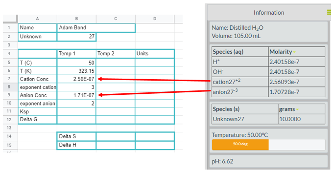
You need to be sure the species and solid viewers are activated so you can read the concentrations of the unknowns and make sure a solid is present. Figure \(\PageIndex{1}\) is a screen shot for unknown 27.  Note the cation is identified as "cation27" and has a charge of +2, while the anion is identified as "anion27" and has a charge of -3.  So this could be a compound like barium phosphate (Ba₃(PO₄)₂).

Figure \(\PageIndex{1}\): Copy and Paste Caption here. (Copyright; author via source)

Using the following Virtual lab to fill in the answers on your Google Worksheet.

 

Google Sheets

Each student works on their own Google Sheet where they submit their results.  They need to read the temperature and concentrations of cation and anion from the virtual lab, and calculate the exponent of the equilibrium constant expression for both the cation and anion (use the number 1 if the value is one).

Figure \(\PageIndex{1}\): Copy and Paste Caption here. (Copyright; author via source)