
14.4: Effect of Concentration on Reaction Rate
- Page ID
- 60727

\( \newcommand{\vecs}[1]{\overset { \scriptstyle \rightharpoonup} {\mathbf{#1}} } \)
\( \newcommand{\vecd}[1]{\overset{-\!-\!\rightharpoonup}{\vphantom{a}\smash {#1}}} \)
\( \newcommand{\id}{\mathrm{id}}\) \( \newcommand{\Span}{\mathrm{span}}\)
( \newcommand{\kernel}{\mathrm{null}\,}\) \( \newcommand{\range}{\mathrm{range}\,}\)
\( \newcommand{\RealPart}{\mathrm{Re}}\) \( \newcommand{\ImaginaryPart}{\mathrm{Im}}\)
\( \newcommand{\Argument}{\mathrm{Arg}}\) \( \newcommand{\norm}[1]{\| #1 \|}\)
\( \newcommand{\inner}[2]{\langle #1, #2 \rangle}\)
\( \newcommand{\Span}{\mathrm{span}}\)
\( \newcommand{\id}{\mathrm{id}}\)
\( \newcommand{\Span}{\mathrm{span}}\)
\( \newcommand{\kernel}{\mathrm{null}\,}\)
\( \newcommand{\range}{\mathrm{range}\,}\)
\( \newcommand{\RealPart}{\mathrm{Re}}\)
\( \newcommand{\ImaginaryPart}{\mathrm{Im}}\)
\( \newcommand{\Argument}{\mathrm{Arg}}\)
\( \newcommand{\norm}[1]{\| #1 \|}\)
\( \newcommand{\inner}[2]{\langle #1, #2 \rangle}\)
\( \newcommand{\Span}{\mathrm{span}}\) \( \newcommand{\AA}{\unicode[.8,0]{x212B}}\)
\( \newcommand{\vectorA}[1]{\vec{#1}} % arrow\)
\( \newcommand{\vectorAt}[1]{\vec{\text{#1}}} % arrow\)
\( \newcommand{\vectorB}[1]{\overset { \scriptstyle \rightharpoonup} {\mathbf{#1}} } \)
\( \newcommand{\vectorC}[1]{\textbf{#1}} \)
\( \newcommand{\vectorD}[1]{\overrightarrow{#1}} \)
\( \newcommand{\vectorDt}[1]{\overrightarrow{\text{#1}}} \)
\( \newcommand{\vectE}[1]{\overset{-\!-\!\rightharpoonup}{\vphantom{a}\smash{\mathbf {#1}}}} \)
\( \newcommand{\vecs}[1]{\overset { \scriptstyle \rightharpoonup} {\mathbf{#1}} } \)
\( \newcommand{\vecd}[1]{\overset{-\!-\!\rightharpoonup}{\vphantom{a}\smash {#1}}} \)
\(\newcommand{\avec}{\mathbf a}\) \(\newcommand{\bvec}{\mathbf b}\) \(\newcommand{\cvec}{\mathbf c}\) \(\newcommand{\dvec}{\mathbf d}\) \(\newcommand{\dtil}{\widetilde{\mathbf d}}\) \(\newcommand{\evec}{\mathbf e}\) \(\newcommand{\fvec}{\mathbf f}\) \(\newcommand{\nvec}{\mathbf n}\) \(\newcommand{\pvec}{\mathbf p}\) \(\newcommand{\qvec}{\mathbf q}\) \(\newcommand{\svec}{\mathbf s}\) \(\newcommand{\tvec}{\mathbf t}\) \(\newcommand{\uvec}{\mathbf u}\) \(\newcommand{\vvec}{\mathbf v}\) \(\newcommand{\wvec}{\mathbf w}\) \(\newcommand{\xvec}{\mathbf x}\) \(\newcommand{\yvec}{\mathbf y}\) \(\newcommand{\zvec}{\mathbf z}\) \(\newcommand{\rvec}{\mathbf r}\) \(\newcommand{\mvec}{\mathbf m}\) \(\newcommand{\zerovec}{\mathbf 0}\) \(\newcommand{\onevec}{\mathbf 1}\) \(\newcommand{\real}{\mathbb R}\) \(\newcommand{\twovec}[2]{\left[\begin{array}{r}#1 \\ #2 \end{array}\right]}\) \(\newcommand{\ctwovec}[2]{\left[\begin{array}{c}#1 \\ #2 \end{array}\right]}\) \(\newcommand{\threevec}[3]{\left[\begin{array}{r}#1 \\ #2 \\ #3 \end{array}\right]}\) \(\newcommand{\cthreevec}[3]{\left[\begin{array}{c}#1 \\ #2 \\ #3 \end{array}\right]}\) \(\newcommand{\fourvec}[4]{\left[\begin{array}{r}#1 \\ #2 \\ #3 \\ #4 \end{array}\right]}\) \(\newcommand{\cfourvec}[4]{\left[\begin{array}{c}#1 \\ #2 \\ #3 \\ #4 \end{array}\right]}\) \(\newcommand{\fivevec}[5]{\left[\begin{array}{r}#1 \\ #2 \\ #3 \\ #4 \\ #5 \\ \end{array}\right]}\) \(\newcommand{\cfivevec}[5]{\left[\begin{array}{c}#1 \\ #2 \\ #3 \\ #4 \\ #5 \\ \end{array}\right]}\) \(\newcommand{\mattwo}[4]{\left[\begin{array}{rr}#1 \amp #2 \\ #3 \amp #4 \\ \end{array}\right]}\) \(\newcommand{\laspan}[1]{\text{Span}\{#1\}}\) \(\newcommand{\bcal}{\cal B}\) \(\newcommand{\ccal}{\cal C}\) \(\newcommand{\scal}{\cal S}\) \(\newcommand{\wcal}{\cal W}\) \(\newcommand{\ecal}{\cal E}\) \(\newcommand{\coords}[2]{\left\{#1\right\}_{#2}}\) \(\newcommand{\gray}[1]{\color{gray}{#1}}\) \(\newcommand{\lgray}[1]{\color{lightgray}{#1}}\) \(\newcommand{\rank}{\operatorname{rank}}\) \(\newcommand{\row}{\text{Row}}\) \(\newcommand{\col}{\text{Col}}\) \(\renewcommand{\row}{\text{Row}}\) \(\newcommand{\nul}{\text{Nul}}\) \(\newcommand{\var}{\text{Var}}\) \(\newcommand{\corr}{\text{corr}}\) \(\newcommand{\len}[1]{\left|#1\right|}\) \(\newcommand{\bbar}{\overline{\bvec}}\) \(\newcommand{\bhat}{\widehat{\bvec}}\) \(\newcommand{\bperp}{\bvec^\perp}\) \(\newcommand{\xhat}{\widehat{\xvec}}\) \(\newcommand{\vhat}{\widehat{\vvec}}\) \(\newcommand{\uhat}{\widehat{\uvec}}\) \(\newcommand{\what}{\widehat{\wvec}}\) \(\newcommand{\Sighat}{\widehat{\Sigma}}\) \(\newcommand{\lt}{<}\) \(\newcommand{\gt}{>}\) \(\newcommand{\amp}{&}\) \(\definecolor{fillinmathshade}{gray}{0.9}\)Rate Law
The Rate Law is a power function that describes the effect of the concentration of the reactants on the rate of reaction for a reaction occurring at constant temperature.
If there is only one reactant it has the form of
\[A \rightarrow Products \\ R=k[A]^m\]
Using the convention introduced in section 14.2.1 of this chapter, R is the rate of reaction, [A]represent the concentration of reactant A, typically in units of molarity (moles reactant per liter), and m is a constant, the order of reaction with respect to A. So the rate law is a power function that describes how R (the dependent variable) depends on the concentration of A (the independent variable)
If there are two reactants, say A and B, then the relationship is extended to two independent variables, each with their own order of reaction
\[A + B \ \rightarrow Products \\ R=k[A]^m[B]^n\]
Each additional reaction contributes an additional independent variable to this power function, each with its own order of reaction, and so three reactants would have the following relationship
\[A + B + C \ \rightarrow Products \\ R=k[A]^m[B]^n[C]^p\]
Students often get confused with the "reaction rate" and the "rate constant" and it is good to take a look at each part of the rate law before proceeding.
The variables
In the rate law the rate is dependent on the reaction concentrations so:
- R the reaction rate is the dependent variable representing the change in concentration of any species related to time and can be expressed in terms of either reactants or products. This is often confusing for students as you can describe the rate by the consumption of any reactant or the production of any product, and these various rates are all related, as described in section 14.2.3 . If you know the rate of one species, you can calculate the rate of any other, just remember that over time reactants decrease in concentration (have a negative sign) and products increase in concentration.
- The concentrations [A], [B], [C], ... are the independent variables (remember [ ] describes concentration). As the concentration of each reactant can be varied, the number of independent variables equals the number of reactant species. Typically the higher the concentration the faster the rate, but this is not always true, and depends on the values of the constants in the rate law.
The Constants
- m,n,p... the power of the power function with respect to each independent variable are called the "orders of reaction" They are typically integers and have values starting with zero (in this class we will consider them always to be integers). Each reactant has its own order of reaction, typically represented with a lower case letter. Lets look at the orders of reaction for a single independent variable [A], which has the order of reaction m
\[R=k[A]^m\]- m = 0 (Zero Order Reaction): Here the rate is not affected by the concentration and if you were to double the concentration the rate would not change.
\[R=k\] - m = 1 (First Order Reaction): This is a linear relationship and if you double the concentration you double the rate of reaction
\[R=k[A]\] - m=2 (Second Order Reaction): This is a squared relationship and if you double the concentration the rate quadruples
\[R=k[A]^2\] - m=3 (Third Order Reaction): This is a cubed relationship and if you double the concentration it goes eight times faster.
\[R=k[A]^3\] - m=n (nth Order Reaction): Very few reactants have orders higher than third, but if you double the concentration it goes 2n times faster.
\[R=k[A]^n\]
- m = 0 (Zero Order Reaction): Here the rate is not affected by the concentration and if you were to double the concentration the rate would not change.
OVERALL ORDER of REACTION (\(\Theta\)):
We will use the Greek symbol Theta \(\Theta\) to describe the sum (\(\Sigma\)) of the order of reaction for all reactants in a chemical reaction
- \(\Theta\) = m+n for two reactants where (\(R=k[A]^m[B]^n\))
- \(\Theta\) = m+n+p for three reactants where (\(R=k[A]^m[B]^n[C]^p\))
- k is the rate constant. Actually, as we will see in section 14.6, k is not really a constant but a function of temperature. But right now we are looking at the concentration dependence of the reaction and will not consider the temperature effect. Also,the convention is to use e a lower case k for rate constants, as in the next chapter we will introduce the equilibrium constant (K), and will use that to distinguish it from the rate constant. Likewise, we will use t for time T for temperature.
The units of k depend on \(\Theta\) the overall order of reaction (see table below). Lets look at the units without identifying the species. The rate has units of concentration/time \(R=\frac{\Delta[concentration]}{\Delta time}\) and each concentration has units of concentration to the power of its order of reaction, so in terms of units we could write:
\[\frac{[concentration]}{time}=k[concentration]^{\theta}\]
so dimensionally speaking the units of k would be
\[k=\frac{\frac{[concentration]}{time}}{[concentration]^{\theta}} = \frac{[concentration^{1-\Theta}]}{time}\]
So for a reaction where concentration was in molarity and time in seconds, the units of k ar
\[\frac{M^{(1-\Theta)}}{second}\]
Let's summarize this in the following table for the reaction, where A, B and C are reactants, and the order of reaction is m for A, n for B and p for C, with an overall order \(\Theta\)= m+n+p
\[\text{rate}=k[A]^m[B]^n[C]^p\]
| Rate law | (m) | (n) | (p) | Overall order \(\Theta\) |
|---|---|---|---|---|
| \(\text{rate}=k\) | 0 | 0 | 0 | 0 |
| \(\text{rate}=k[A]\) | 1 | 0 | 0 | 1 |
| \(\text{rate}=k[A]^2\) | 2 | 0 | 0 | 2 |
| \(\text{rate}=k[A][B]\) | 1 | 1 | 0 | 2 |
| \(\text{rate}=k[A]^2[B]\) | 2 | 1 | 0 | 3 |
| \(\text{rate}=k[A][B][C]\) | 1 | 1 | 1 | 3 |
It should be noted that most chemical reactions are zero, first or second order.
Experimental Determination of Rate Law
We know the dependent variable (R) is a function of the independent variable, and on a piece of graph paper can plot out this relationship with R on the Y-axis and the independent variable [reactant concentration] on the the x-axis. The problem is, every reactant is an independent variable, and you can only graph one independent variable on a two dimensional plot. So if there is more than one reactant, you have to reduce the number of independent variables to one. If we assume the orders of reaction for each reactant are independent of each other (m does not change n), we can run a series of experiments where we vary one reactant concentration at a time to determine its order of reaction, while keeping all others constant. By successively doing this for all reactants we can determine the order of reaction for all species.
This lesson will start by solving the single reactant rate law. Then show how to reduce multi-reactant problems to single reactant problems. We will also introduce two different techniques for solving these. First the Ratio (Two State) Technique, which works well for "precise data", and then the graphing technique, which needs to be used when the data is unprecise. In the lab we will run an experiment where we have to use the graphing technique.
Single Reactant Rate Law
Consider the reaction:
\[A \rightarrow B\]
The Rate Law for the above is:
\[R=k[A]^{m}\]
We need to solve for k and m. There are two approaches. If we have real good data, we can use the two state method. If we have bad data, like the data you use in lab, we will need to use the graphing technique. Note:, since "m" is in an exponent, we will need to use logarithms, and the relationship logab = bloga.
Exercise \(\PageIndex{1}\)
Solve the following equation for m.
\[56.3=32\left ( 0.45^{m} \right )\]
- Answer
-
\[0.45^m=\frac{56.3}{32} \\
log0.45^m=log\frac{56.3}{32} \\
mlog0.45=log\frac{56.3}{32} \\
m=\frac{log\frac{56.3}{32}}{log0.45} =\frac{0.24536}{-0.34679}= -0.7075 \nonumber\]
Graphing Technique
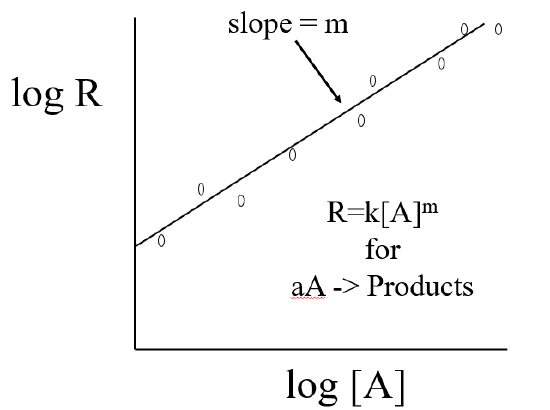
Because the rate law is a power function we need to use logarithms to determine the order of reaction. First take the log of both sides
\[logR=logk[A]^{m}\]
Using the relationship lnab = lna + lnb gives
\[ logR=logk + log[A]^{m} \]
then using the relationship \(log[A]^b=blog[A]\) and rearranging gives
\[ logR=mlog[A] + logk \]
which has the form of a straight line with slope=m
y=mx+b
Where, y=logR, x=log[A] and b=logk
To get k you take the antilog of b
\[k=10^b\]
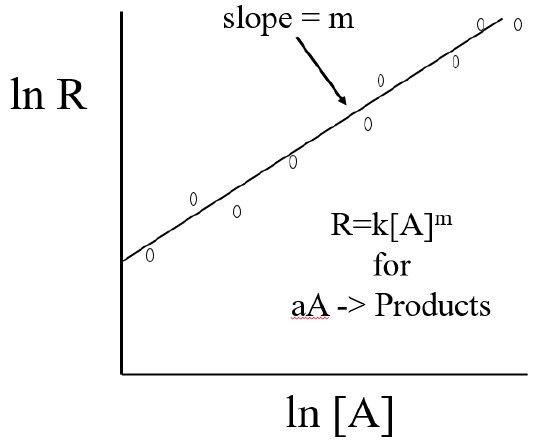
Note, you could have used any base to the log scale and ploted
\[lnR=mln[A]+lnk\]
in which case Y=lnR, X = ln[A] and b= lnk, so k=eb.
Two State Technique
If your data is exact, and all the data is on the line, you can use the two state approach, that is you can simply use the data from only two measurements. So we run an experiment with a known concentration and measure the initial rate (state 1). Now we change the concentration and measure the initial rate (state 2). We divide state one by state 2 as we have done in the other two-state problems like the ideal gas and Henry's Law calculations.
\[\begin{align} \frac{R_{1}}{R_{2}} & = \frac{k[A_{1}]^{m}}{k[A_{2}]^{m}} \nonumber \\ \nonumber \\ \frac{R_{1}}{R_{2}} & =\left ( \frac{[A_{1}]}{[A_{2}]} \right )^{m} \nonumber \\ \nonumber \\ \log \left ( \frac{R_{1}}{R_{2}} \right ) & =m\log \left ( \frac{[A_{1}]}{[A_{2}]} \right ) \nonumber \\ \nonumber \\ m & =\frac{\log\left ( \frac{R_{1}}{R_{2}} \right )}{\log\left ( \frac{[A_{1}]}{[A_{2}]} \right )} \end{align} \]
Once we calculate m, we can substitute back into one of the states and solve for k (see following worked example)
Multi Reactant Systems
Lets look at a system involving three reactants,
\[A + B + C \rightarrow Products \\ R=k[A]^m[B]^n[C]^p\]
In the above equation we have on dependent variable (the rate), which has a value that depends on three independent variables, the concentrations of chemical species "A" and "B", and "C". Can you think of an equation from General Chemistry 1 that had four variables? How about the Ideal Gas Law? If you review section 10.2 Gas Laws, you will see that historically a series of "empirical gas laws" were experimentally developed that were in essence the ideal gas law with two of the four variables held constant.
- Boyle's Law: P=k\(\frac{1}{V}\) (PV=nRT at constant n,T)
- Gay-Lussacs Law: P=k'T (PV=nRT at constant n,V)
- Charles's Law: V=k''T (PV=nRT at constant n,P)
- Avogadro's Law V=k'''n (PV=nRT at consant P,T)
We are going to take the same strategy, although there is a slight difference between the rate law with three reactants and the ideal gas law, in that the ideal gas law was an equation of state and all variables were equal, whereas here the rate is a dependent variable and the concentrations are independent. So you design a series of experiments where two of the concentrations are constant and vary the third to see how it affects the rate. You then sequentially repeat this for the remaining two independent variables, so in essence you need to run three sets of experiments, where in each set only one of the concentrations vary. If your data is exact, you do not need to make a graph, but can use the two state approach.
Table 13.3.3 Rate Data for a Hypothetical Reaction of the Form A + B → Products
| Experiment | [A] (M) | [B] (M) | [C](M) | Initial Rate (M/s) |
|---|---|---|---|---|
| 1 | 0.10 | 0.10 | 0.10 | 0.00475 |
| 2 | 0.20 | 0.10 | 0.10 | 0.019 |
| 3 | 0.20 | 0.20 | 0.10 | 0.152 |
| 4 | 0.20 | 0.10 | 0.20 | 0.038 |
- Step 1: Determine m by running set of experiments at constant [B] and [C] constant.
This can be done with experiments 1 and 2. TRICK: place the larger concentration in the numerator
Lets start by looking at the entire rate law
\[ \frac{rate_{2}}{rate_{1}}= \frac{k[A_2]^m[B_2]^n[C_2]^p}{k[A_1]^m[B_1]^n[C_1]^p} =\frac{{\color{Red} \cancel{k}}[A_2]^m[0.1]^n[0.1]^p}{{\color{Red} \cancel{k}}[A_1]^m[0.1]^n[0.1]^p} \nonumber\]
\[\frac{R_2}{R_1}=\left ( \frac{A_2}{A_1} \right )^m {\color{Blue} \cancel{\left ( \frac{0.1}{0.1} \right )^n}} {\color{Red} \cancel{\left ( \frac{0.1}{0.1} \right )^p}} \nonumber\]
\[\frac{R_2}{R_1}= \left ( \frac{A_2}{A_1} \right )^m \\ \frac{0.019{\color{Red} \cancel{M}}}{0.00475{\color{Red} \cancel{M}}} =\left ( \frac{.20 {\color{Red} \cancel{M/s}}}{.10{\color{Red} \cancel{M/s}}} \right )^m \\ \;\\4=2^m \\ \;\\m=2 \]
Step 2: Determine n by running set of experiments at constant [A] and [C] constant
Experiments 3 and 2
\[\frac{R_3}{R_2}=\left ( \frac{B_3}{B_2} \right )^n \\ \frac{0.152{\color{Red} \cancel{M}}}{0.019{\color{Red} \cancel{M}}} =\left ( \frac{.20 {\color{Red} \cancel{M/s}}}{.10{\color{Red} \cancel{M/s}}} \right )^n\\ \; \\8=2^m \\ \; \\n=3 \]
NOTE: Dividing R2 by R3 (not place the larger concentration in the numerator) would have given 0.125=0.50n for the second to last step and a student may not have recognized that as 1/8=(1/2)n, in which case they would need to take the log of both sides to find n.
\[\frac{R_2}{R_3}=\left ( \frac{B_2}{B_3} \right )^n \\ \frac{0.019{\color{Red} \cancel{M}}}{0.152{\color{Red} \cancel{M}}} =\left ( \frac{0.10 {\color{Red} \cancel{M/s}}}{0.20{\color{Red} \cancel{M/s}}} \right )^n\\ \; \\0.125=0.50^m \Rightarrow log(0.125)=log(0.50)^n =nlog(0.50)\\ \; \\n=\frac{log0.125}{log0.50} =\frac{-0.90309}{-0.30103} =3 \]
Step 3: Determine p by running set of experiments at constant [A] and [B] constant
Experiments 4 and 2
\[\frac{R_4}{R_2}=\left ( \frac{C_4}{C_2} \right )^p \\ \frac{0.038{\color{Red} \cancel{M}}}{0.019{\color{Red} \cancel{M}}} =\left ( \frac{.20 {\color{Red} \cancel{M/s}}}{.10{\color{Red} \cancel{M/s}}} \right )^n\\ \; \\4=2^p \\ \; \\p=2 \]
Step 4: Determine k, the rate constant
\[k=\frac{R}{[A]^m[B]^n][C]^p}=\frac{0.00475M/s}{[0.1M]^2[0.1M]^3[0.1M]}=4800s^{-1}M^{-5}\]
Note
In the above problems we changed the concentration by orders of 2. This made the math very easy and you could have just looked and seen the order of reaction. But also, it is very easy to change the concentration of a reactant by 2. You simply take some of it and dilute in half, and now the original solution is twice that of the diluted.
- In going from experiment 1 to 2 we doubled the concentration of [A] at constant [B], [C] and the reaction went 4 times as fast, so the order with respect to A is 2, as 22=4.
- In going from experiment 2 to 3 we doubled the concentration of [B] at constant [A], [C] and the reaction went 8 times as fast, so the order with respect to B is 3, as 23=8.
- In going from experiment 2 to 4 we doubled the concentration of [C] at constant [A], [B] and the reaction went 4 times as fast, so the order with respect to C is 2, as 21=2.
Exercise \(\PageIndex{2}\)
Using the initial rates method and the experimental data, determine the rate law and the value of the rate constant for this reaction:
\[\ce{2NO}(g)+\ce{Cl2}(g)⟶\ce{2NOCl}(g)\]
| Trial | [NO] (mol/L) | [Cl2] (mol/L) | \(−\dfrac{Δ[\ce{NO}]}{Δt}\mathrm{(mol\:L^{−1}\:s^{−1})}\) |
|---|---|---|---|
| 1 | 0.10 | 0.10 | 0.00300 |
| 2 | 0.10 | 0.15 | 0.00450 |
| 3 | 0.15 | 0.10 | 0.00675 |
- Answer
-
Solution
The rate law for this reaction will have the form:
\[\ce{rate}=k[\ce{NO}]^m[\ce{Cl2}]^n\]1. Determine the value of m (at constant [Cl2]):
\[\dfrac{\ce{rate}_x}{\ce{rate}_y}=\dfrac{k[\ce{NO}]^m_x[\ce{Cl2}]^n_x}{k[\ce{NO}]^m_y[\ce{Cl2}]^n_y}\]Using the third trial and the first trial:
\[\mathrm{\dfrac{rate\: 3}{rate\: 1}}=\dfrac{0.00675}{0.00300}=\dfrac{\cancel{k}(0.15)^m\cancel{(0.10)^n}}{\cancel{k}(0.10)^m \cancel{(0.10)^n}}\]After canceling equivalent terms in the numerator and denominator, we are left with:
\[\dfrac{0.00675}{0.00300}=\dfrac{(0.15)^m}{(0.10)^m}\]which simplifies to:
\[2.25=(1.5)^m\]We can use the log of any base to determine the value of the exponent m, (we used base 10 in the worked out example above, and will use natural logs here).
\(\begin{align}
\ln(2.25)&=m\ln(1.5) \\
m & =\dfrac{\ln(2.25)}{\ln(1.5)} \\ m&=2
\end{align}\)We can confirm the result easily, since:
\(1.5^2=2.25\) 2. Determine the value of n (at constant [NO]).
\[\mathrm{\dfrac{rate\: 2}{rate\: 1}}=\dfrac{0.00450}{0.00300}=\dfrac{\cancel{k(0.10)^m}(0.15)^n}{\cancel{k(0.10)^m}(0.10)^n}\]Cancelation gives:
\[\dfrac{0.0045}{0.0030}=\dfrac{(0.15)^n}{(0.10)^n}\]which simplifies to:
\[1.5=(1.5)^n\] Thus n must be 1, and the form of the rate law is:
\[\ce{Rate}=k[\ce{NO}]^m[\ce{Cl2}]^n=k[\ce{NO}]^2[\ce{Cl2}]\]3. Determine the numerical value of the rate constant k with appropriate units. Since the overall order of reaction is three, the units are M-2s-1, l2mol-2s-1. To determine the value of k once the rate law expression has been solved, simply plug in values from any experiment, we will use the first experimental trial because the math is easiest, and solve for k:
\(\begin{align}
\mathrm{0.00300\:mol\:L^{−1}\:s^{−1}}&=k\mathrm{(0.10\:mol\:L^{−1})^2(0.10\:mol\:L^{−1})^1}\\
k&=\mathrm{3.0\:mol^{−2}\:L^2\:s^{−1}}
\end{align}\)
In Class Activity
ADAPT \(\PageIndex{1}\)
Test Yourself
Homework: Section 14.4
Query \(\PageIndex{1}\)
Query \(\PageIndex{2}\)
Query \(\PageIndex{3}\)
Robert E. Belford (University of Arkansas Little Rock; Department of Chemistry). The breadth, depth and veracity of this work is the responsibility of Robert E. Belford, rebelford@ualr.edu. You should contact him if you have any concerns. This material has both original contributions, and content built upon prior contributions of the LibreTexts Community and other resources, including but not limited to:
- Liliane Poirot