14.5: Integrated Rate Law
- Page ID
- 60728
\( \newcommand{\vecs}[1]{\overset { \scriptstyle \rightharpoonup} {\mathbf{#1}} } \)
\( \newcommand{\vecd}[1]{\overset{-\!-\!\rightharpoonup}{\vphantom{a}\smash {#1}}} \)
\( \newcommand{\id}{\mathrm{id}}\) \( \newcommand{\Span}{\mathrm{span}}\)
( \newcommand{\kernel}{\mathrm{null}\,}\) \( \newcommand{\range}{\mathrm{range}\,}\)
\( \newcommand{\RealPart}{\mathrm{Re}}\) \( \newcommand{\ImaginaryPart}{\mathrm{Im}}\)
\( \newcommand{\Argument}{\mathrm{Arg}}\) \( \newcommand{\norm}[1]{\| #1 \|}\)
\( \newcommand{\inner}[2]{\langle #1, #2 \rangle}\)
\( \newcommand{\Span}{\mathrm{span}}\)
\( \newcommand{\id}{\mathrm{id}}\)
\( \newcommand{\Span}{\mathrm{span}}\)
\( \newcommand{\kernel}{\mathrm{null}\,}\)
\( \newcommand{\range}{\mathrm{range}\,}\)
\( \newcommand{\RealPart}{\mathrm{Re}}\)
\( \newcommand{\ImaginaryPart}{\mathrm{Im}}\)
\( \newcommand{\Argument}{\mathrm{Arg}}\)
\( \newcommand{\norm}[1]{\| #1 \|}\)
\( \newcommand{\inner}[2]{\langle #1, #2 \rangle}\)
\( \newcommand{\Span}{\mathrm{span}}\) \( \newcommand{\AA}{\unicode[.8,0]{x212B}}\)
\( \newcommand{\vectorA}[1]{\vec{#1}} % arrow\)
\( \newcommand{\vectorAt}[1]{\vec{\text{#1}}} % arrow\)
\( \newcommand{\vectorB}[1]{\overset { \scriptstyle \rightharpoonup} {\mathbf{#1}} } \)
\( \newcommand{\vectorC}[1]{\textbf{#1}} \)
\( \newcommand{\vectorD}[1]{\overrightarrow{#1}} \)
\( \newcommand{\vectorDt}[1]{\overrightarrow{\text{#1}}} \)
\( \newcommand{\vectE}[1]{\overset{-\!-\!\rightharpoonup}{\vphantom{a}\smash{\mathbf {#1}}}} \)
\( \newcommand{\vecs}[1]{\overset { \scriptstyle \rightharpoonup} {\mathbf{#1}} } \)
\( \newcommand{\vecd}[1]{\overset{-\!-\!\rightharpoonup}{\vphantom{a}\smash {#1}}} \)
\(\newcommand{\avec}{\mathbf a}\) \(\newcommand{\bvec}{\mathbf b}\) \(\newcommand{\cvec}{\mathbf c}\) \(\newcommand{\dvec}{\mathbf d}\) \(\newcommand{\dtil}{\widetilde{\mathbf d}}\) \(\newcommand{\evec}{\mathbf e}\) \(\newcommand{\fvec}{\mathbf f}\) \(\newcommand{\nvec}{\mathbf n}\) \(\newcommand{\pvec}{\mathbf p}\) \(\newcommand{\qvec}{\mathbf q}\) \(\newcommand{\svec}{\mathbf s}\) \(\newcommand{\tvec}{\mathbf t}\) \(\newcommand{\uvec}{\mathbf u}\) \(\newcommand{\vvec}{\mathbf v}\) \(\newcommand{\wvec}{\mathbf w}\) \(\newcommand{\xvec}{\mathbf x}\) \(\newcommand{\yvec}{\mathbf y}\) \(\newcommand{\zvec}{\mathbf z}\) \(\newcommand{\rvec}{\mathbf r}\) \(\newcommand{\mvec}{\mathbf m}\) \(\newcommand{\zerovec}{\mathbf 0}\) \(\newcommand{\onevec}{\mathbf 1}\) \(\newcommand{\real}{\mathbb R}\) \(\newcommand{\twovec}[2]{\left[\begin{array}{r}#1 \\ #2 \end{array}\right]}\) \(\newcommand{\ctwovec}[2]{\left[\begin{array}{c}#1 \\ #2 \end{array}\right]}\) \(\newcommand{\threevec}[3]{\left[\begin{array}{r}#1 \\ #2 \\ #3 \end{array}\right]}\) \(\newcommand{\cthreevec}[3]{\left[\begin{array}{c}#1 \\ #2 \\ #3 \end{array}\right]}\) \(\newcommand{\fourvec}[4]{\left[\begin{array}{r}#1 \\ #2 \\ #3 \\ #4 \end{array}\right]}\) \(\newcommand{\cfourvec}[4]{\left[\begin{array}{c}#1 \\ #2 \\ #3 \\ #4 \end{array}\right]}\) \(\newcommand{\fivevec}[5]{\left[\begin{array}{r}#1 \\ #2 \\ #3 \\ #4 \\ #5 \\ \end{array}\right]}\) \(\newcommand{\cfivevec}[5]{\left[\begin{array}{c}#1 \\ #2 \\ #3 \\ #4 \\ #5 \\ \end{array}\right]}\) \(\newcommand{\mattwo}[4]{\left[\begin{array}{rr}#1 \amp #2 \\ #3 \amp #4 \\ \end{array}\right]}\) \(\newcommand{\laspan}[1]{\text{Span}\{#1\}}\) \(\newcommand{\bcal}{\cal B}\) \(\newcommand{\ccal}{\cal C}\) \(\newcommand{\scal}{\cal S}\) \(\newcommand{\wcal}{\cal W}\) \(\newcommand{\ecal}{\cal E}\) \(\newcommand{\coords}[2]{\left\{#1\right\}_{#2}}\) \(\newcommand{\gray}[1]{\color{gray}{#1}}\) \(\newcommand{\lgray}[1]{\color{lightgray}{#1}}\) \(\newcommand{\rank}{\operatorname{rank}}\) \(\newcommand{\row}{\text{Row}}\) \(\newcommand{\col}{\text{Col}}\) \(\renewcommand{\row}{\text{Row}}\) \(\newcommand{\nul}{\text{Nul}}\) \(\newcommand{\var}{\text{Var}}\) \(\newcommand{\corr}{\text{corr}}\) \(\newcommand{\len}[1]{\left|#1\right|}\) \(\newcommand{\bbar}{\overline{\bvec}}\) \(\newcommand{\bhat}{\widehat{\bvec}}\) \(\newcommand{\bperp}{\bvec^\perp}\) \(\newcommand{\xhat}{\widehat{\xvec}}\) \(\newcommand{\vhat}{\widehat{\vvec}}\) \(\newcommand{\uhat}{\widehat{\uvec}}\) \(\newcommand{\what}{\widehat{\wvec}}\) \(\newcommand{\Sighat}{\widehat{\Sigma}}\) \(\newcommand{\lt}{<}\) \(\newcommand{\gt}{>}\) \(\newcommand{\amp}{&}\) \(\definecolor{fillinmathshade}{gray}{0.9}\)Introduction
Consider the following generic reaction of chemical species A turning into species B,
\[\begin{align} &A\rightarrow B \nonumber \\ \nonumber \\ R= & -\frac{\Delta [A]}{\Delta t}= \frac{\Delta [B]}{\Delta t}=k[A]^{m} \end{align}\]
The above equation is a power function relating the rate of reaction to the concentration, with the nature of that relationship being defined by the order of reaction. Yet the rate itself is a function of concentration \(R= \frac{\Delta [ \; \; ]}{\Delta t}\), where [ ] represents the concentration of some species (reactant or product). If we express the rate law as the consumption of the reactant [A], the we have one equation with two variables, which we could graph, that is [A] is a function of t.
\[-\frac{\Delta [A]}{\Delta t}=k[A]^{m} \\ \; \text{rearranging to we can look at how the concentration changes over time give"} \\ \; \\ \frac{\Delta[A]}{[A]^m}=-k\Delta t\]
The problem is that it is the change in A as a function of the change in t, which requires calculus to solve, and calculus is not a prerequisite to this course. So we are going to memorize the algebraic solutions of the integrated rate law for zero, first and second order reactions.
Optional Background material
For those of you who have had calculus, or wish to get a bearing on where these equations come from, we need to start with the concept of the derivative, which is the rate at an instant in time, that is, as \(\Delta\)t approaches zero.
\[ \lim_{\Delta t \rightarrow 0} \dfrac{\Delta [A]}{\Delta t}=\dfrac{d[A]}{dt} \label{eq3}\]
the rate law becomes.
\[ \frac{d[A]}{dt}=-k[A]^{m} \label{eq4} \]
which from calculus, you can separate the variables and integrate
\[ \int \frac{d[A]}{[A]^{m}} = -\int k\,dt \label{eq4B}\]
There is one solution to the right hand side of Equation \ref{eq4B}
\[- \int_{t=0}^{t}kdt=-k(t-0)=-kt \label{eq5}\]
There are two solutions to the left part of Equation \ref{eq4B}. Note, Equation \ref{eq6} expresses the equation the way it normally is expressed in calculus classes (the dependent variable is in the numenator [A]n), but in Equation \ref{eq4B} it is in the denominator ([A]-m), and so in comparing these equations \(m = -n\).
\[ \underbrace { \int_{[A]_0}^{[A]}[A]^{n}d[A]=\frac{1}{n+1}\left ( [A]^{n+1}-[A]_{0}^{n+1} \right )} _{n \neq -1} \label{eq6}\]
when \(n = -1\)
\[\int_{[A]_0}^{[A]}\frac{d[A]}{[A]}=\ln[A]-\ln[A]_0 \label{eq7}\]
The integrated rate laws you need to know are the solutions to the above equation for \(n=0,\,1,\,2\).
Students do not need to know Equation \ref{eq3} - \ref{eq7}. These are just being provided so you know that the integrated rate laws come from calculus solutions to the rate equation. You do need to know the solutions for n = 0,1,2. These are covered in table \(\PageIndex{1}\) of the very next section.
Integrated Rate Laws
Most orders of reaction are zero, first or second. Table \(\PageIndex{1}\) gives the solutions to the integrated rate laws, and you need to know these solutions for zero, first and second order reactions. Note, there is a form of each order of reaction that follows the equation of a straight line (y=mx+b).
| Order | 0 | 1 | 2 |
|---|---|---|---|
| Integrated Rate Law | [A]= -kt + [A]0 | A] = [A]0e-kt or ln[A] = -kt + ln[A]0 | \(\frac{1}{[A]}=kt+\frac{1}{[A]_0}\) |
Implicit in the above equations is that [A], the dependent variable, represents the concentration at any time (t), the independent variable as a function of the rate constant (k) and the initial concentration at t=0, ([A]o). We could write [A] as [A]t to indicate that it is the value of [A] at some time t. The nature of that relationship depends on the order of reaction.
Zero Order Reaction
In zero order reactions the reaction rate is independent of the concentration and the rate is the negative of the rate constant, which has units of concentration/time, like M/sec.
\[Rate=\frac{\Delta [A]}{\Delta{t}}=-k\]
A plot of the concentration of a reactant gives a linear function where the concentration decreases over time at a constant rate.
\[\Large{[A]=−kt+[A]_0} \\ or \\ \; \\ [A]_t=−kt+[A]_0 \\ \; \\ (y=mx + b)\]
Optional Background material
For those of you who have had calculus, or wish to get a bearing on where these equations come from,
\[ \frac{d[A]}{dt} = -k[A]^o =-k \\ \; \\ d[A] = -kdt \\ \; \\ \int_{[A]_0}^{[A]_t}d[A] = - \int_{t=0}^{t}kdt \\ \: \\ [A]_t - [A]_o = -kt -k(0) \\ \; \\ [A]_t = -kt + [A]_o\]
The rate of a zero order reaction does not depend on the concentration of a reactant and it stays constant until all the limiting reagent is completely consumed.
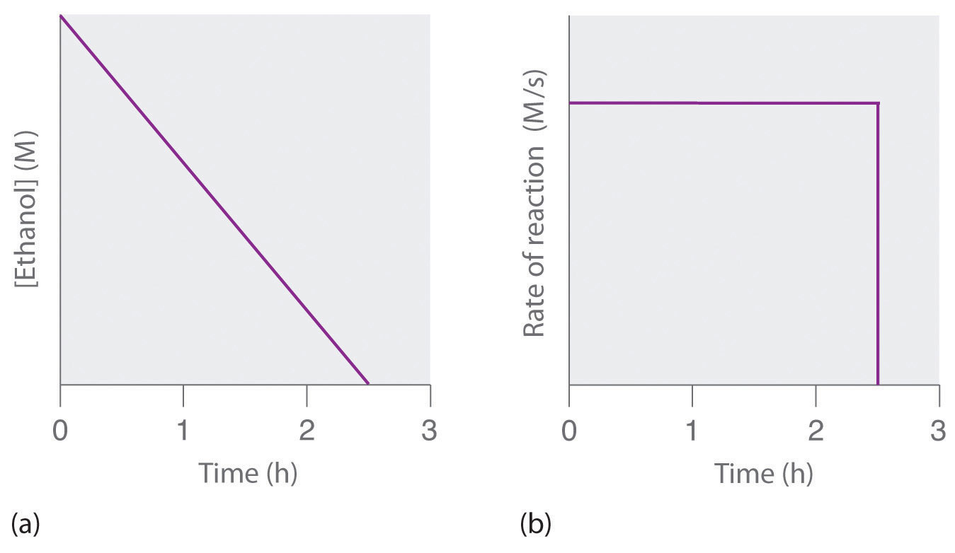
Sometimes it is useful to look at this as:
\[ \underbrace{[A]}_{\text{concentration at time t}}= \underbrace{[A]_0}_{\text{initial concentration}} - \underbrace{kt}_{\text{amount consumed}}\]
Where what you have left ([A]) is what you started with ([A]0) minus the amount consumed over a specified period of time (kt) is the amount consumed. This is very simple math, for example, if a student has $100 in the bank ([A]0] and spends $10/day (k) for three days (t), they have $70 left ([A]).
Zero order reactions are often called pseudo zero order as they are the results of the reaction conditions, typically because a reactant is in excess concentrations compared to others, and always break down to other kinetics as the concentration approaches zero (the rate must change as the reactant concentration approaches zero as it is zero when the concentration is zero). Heterogeneous catalysts like enzymes (next section) are often zero order with respect to substrate (reactant) concentration because there are so few active sites compared to the number of substrate (reactant) molecules that the moment one opens up another substrate molecules is ready to fill it, but this breaks down as the substrate concentration approaches zero.
First Order Reaction
In a first order rate law, the rate of consumption of a reactant is proportional to the consumption of a reactant and the rate constant has units of 1/t, like 1/sec.
\[ Rate = - \dfrac{\Delta [A]}{\Delta t} = k[A]^1 = k[A] \]
rearranging gives,
\[ Rate = \dfrac{\Delta [A]}{\Delta t} = -k[A] \]
A plot of concentration over times gives a first order reaction gives an exponential decay and a plot of the natural log of concentration over times gives a linear decay. Students in general chemistry need to know the following two equations and do not need to know the optional calculus.find the concentration as a function of time we need to apply calculus (Equation \ref{eq6}), and the solution for a first order reaction is:
\[[A]=-kt+[A]_{0} \\ \; \\ (y=mx+b)\]
or
\[ [A] =[A]_{0}e^{-kt}\]
Optional Background material
For those of you who have had calculus, or wish to get a bearing on where these equations come from,
\[ \frac{d[A]}{dt} = -k[A] \\ \; \\ \frac{d[A]}{[A]} = -kdt \\ \; \\ \int_{[A]_0}^{[A]_t} \frac{d[A]}{[A]} = - \int_{t=0}^{t}kdt \\ \: \\ ln[A]_t - ln[A]_o = -kt -k(0) \\ \; \\ ln[A]_t = -kt + ln[A]_o\]
Note
There are two forms of a first order decay, exponential and natural log. The one you use depends on what you are solving for.
- Use Exponential form is solving for [A] or [A]o. (A=Aoe-kt).
- Use Natural log form if solving for k or t. (ln[A] = -kt + ln[A]o).
Closer look at the exponential form and the fraction remaining or consumed
\[\begin{align} [A] & =[A]_{0}e^{-kt} \\ & \therefore \\ \frac{[A]}{[A]_o} &= e^{-kt} \\ & \therefore \\ e^{-kt} &= \text{ fraction of } [A]_o \text{ remaining} \end{align}\]
So one can interpret the exponential form of a first order decay as"
\[\underbrace{[A]}_{\text{concentration remaining}} =\underbrace{[A]_{0}}_{\text{Initial concentration}} \times \underbrace{e^{-kt}}_{\text{fraction remaining}}\]
Since the fraction remaining plust the fraction consumed is equal to 1, we can also calculate the fraction consumed
\[\text{fraction consumed}=1-e^{-kt}\]
Note
The fraction remaining or consumed is independent of the initial concentration, and this is only true for first order reactions.
- Fraction remaining (\(\frac{[A]}{[A]_o}\))=e-kt.
- Fraction consumed (\(\frac{[A]-[A]_o}{[A]_o}\))=1 - e-kt.
This is important because if we know a first order rate constant we can ask questions like how long does it take for half of a sample to be consumed, and that amount of time is independent of the amount of sample we have. In fact this leads to the concept of half lives, which is a common way of describing a first order reaction rate constant. In fact for many people it is more intuitive than the rate constant, but for first order reactions, as we shall see, the half life is directly related to the rate constant, and if you know the half life, you know the rate constant.
Half Lives and First Order Reactions
The half life, is the amount of time it takes for the concentration to be reduced to one half its original value. In the case of a first order reaction, the half life is independent of the concentration.
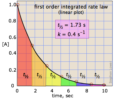
The definition of a half life is the amount of time it takes for a sample to decompose to one half its value. For a single exponential decay this is not a function of the sample size, for other orders of reaction, it is. Mathematically, the half life criteria is
\[at\: \; t=t_{1/2},\: \: [A]=\frac{[A]_{0}}{2} \label{eq14}\]
Substituting the half-life criteria (\([A] = \frac{[A]_o}{2}\))into the first order equation (A=Aoe-kt) gives:
\[ \dfrac{\cancel{[A]_0}}{2} =\cancel{[A]_{0}}e^{-kt_{1/2}}=\frac{\cancel{[A]_o}}{e^{kt_{1/2}}} \label{eq15}\]
cancelling [A]o and taking the reciprocal of both sides gives
\[2=e^{kt_{1/2}}\]
Taking the natural log of both sides and rearranging gives:
\[kt_{1/2}=ln 2=0.693\]
So a table of half lives give you the value of the rate constant (the longer the half life the smaller the rate constant)
\[k=\frac{.693}{t_{1/2}}\]
See Video \(\PageIndex{1}\) for the derivation of Equation \ref{eq16}
So you can write a first order integrated rate law in terms of the rate constant or half life
| First Order Reactions | Exponential Form | Natural Log Form |
|---|---|---|
| Using rate constant | \(\large{A=e^{-kt}}\) | lnA=-kt + lnAo |
| Using half life | \(\large{A=e^{-\frac{0.693}{t_{1/2}}t}}\) | \(lnA= -\frac{0.693}{t_{1/2}}t + lnA_o \) |
Half Lives and Radioactive (Carbon) dating
Carbon-14 undergoes beta (β) decay, in which a neutron is converted to a proton and a high-energy electron that is ejected from the nucleus as a β particle:
\[\underset{\textrm{unstable} \\ \textrm{neutron in} \\ \textrm{nucleus}}{^1_0 \textrm n}\rightarrow \underset{\textrm{proton} \\ \textrm{retained} \\ \textrm{by nucleus}}{^{1}_{1} \textrm p}+\underset{\textrm{beta particle} \\ \textrm{emitted by} \\ \textrm{nucleus}}{^0_{-1} \beta}\label{Eq3} \]
The general reaction for beta decay is therefore
\[\underset{\textrm{parent}}{^A_Z \textrm X}\rightarrow \underset{\textrm{daughter}}{^{A}_{Z+1} \textrm X'}+\underset{\textrm{beta particle}}{^0_{-1} \beta}\label{Eq4} \]
Although beta decay does not change the mass number of the nucleus, it does result in an increase of +1 in the atomic number because of the addition of a proton in the daughter nucleus. Thus beta decay decreases the neutron-to-proton ratio, moving the nucleus toward the band of stable nuclei. For example, carbon-14 undergoes beta decay to form nitrogen-14:
\[^{14}_{6}\textrm{C}\rightarrow ^{14}_{7}\textrm{N}+\,^{0}_{-1}\beta \nonumber \]
The parent and the daughter nuclei have the same mass number, 14, and the sum of the atomic numbers of the products is 6, which is the same as the atomic number of the carbon-14 parent. We will cover nuclear reactions in more detail in chapter 21.
The Carbon-14 Cycle
There are two stable isotopes of carbon, carbon-12 (12C) and carbon-13 (13C), and an unstable radioisotope, carbon-14 (14C), which decays with a half life of 5,730 years. Carbon-14 is continually being generated in the upper atmosphere, where cosmic rays generate free neutrons when they collide with nuclei, and 14C is created when one of these neutrons collides with nitrogen (14N) and in essence knocks out a proton as it is absorbed into the nucleus resulting in carbon-14. The unstable 14C radioisotope (radioactive isotope) eventually emits a beta particle and reverts back to 14N, as described in figure \(\PageIndex{4}\).
In the upper atmosphere
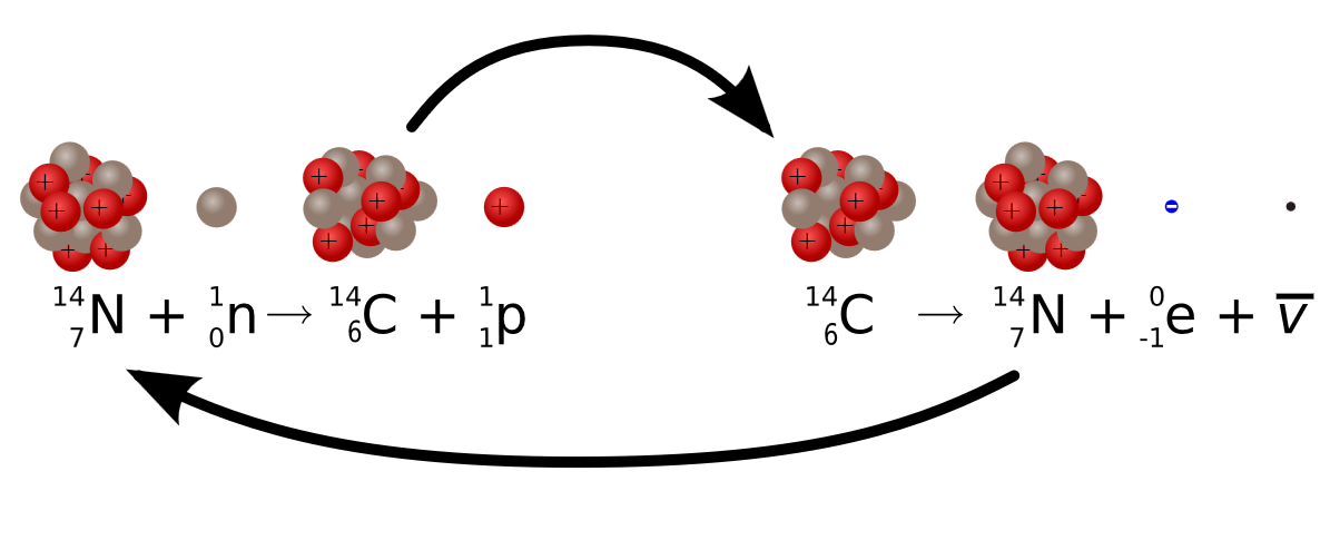
The result of this process is that the ration of 14C to 12C in the atmosphere is constant, and so living plant matter, which absorbs 14C as it uptakes carbon dioxide in the process of photosynthesis has a constant ration of 14C to 12C. Once a plant dies, no more 14C uptake occurs, and the ration decreases as the 14C particles decay to 14N. This is described in figures \(\PageIndex{4}\) and \(\PageIndex{5}\).
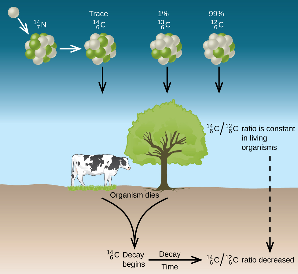
This allows scientists to determine the age of a plant based artifact by assuming that the current ratio of 14C to 12C in the atmosphere was the same when the plant died. In reality, this ratio can fluctuate, for an example, combustion of fossil fuel can increase the atmospheric concentration of "old carbon". It is also important to note that the decay rate of a sample of carbon-14, that is the number of radiating particles, is proportional to the the concentration of carbon-14 in the sample. So the kinetics measure the rate of radiation, which is equal to the rate of change in carbon-14 to nitrogen-14 if one particle is given off each time a nuclei in the sample decays.
Note
Carbon-14 dating takes some assumptions into account, the major one being that the ratio of 14C to 12C is constant from the time the sample died to the time it was tested. This allows one to postulate that living samples have the same ratio as the sample being tested had when it was alive, and so you have a value for the initial decay rate. This assumption may be in error if the atmospheric carbon dioxide differ over the time span, for example the burning of fossil fuels also produce carbon dioxide, but have a different ratio of 14C to 12C to that of respiration, and so their uptake in photosynthesis could result in an alteration of the ratio. In this class we will ignore these effects, and carbon-14 dating is a valuable tool to determine the age of material that was formed through photosynthesis.
Exercise \(\PageIndex{1}\)
In 1988 radiocarbon dating was done on a sample obtained from the Shroud of Turin. At that time, living matter gave off 15.3 disintegrations per minute, and the sample gave off 14.2. How old was the Shroud of Turin in 1988 if the half life of 14C = 5,715 years?
- Answer
-
615 years.
Second Order Reactions
In second order reactions the reaction rate is dependent on the square of the concentration and the rate constant has units of 1/(concentration-time) like M-1s-1.
\[Rate=\frac{\Delta [A]}{\Delta{t}}=-k[A]^2\]
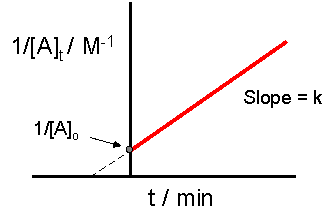
A plot of the reciprocal concentration of a reactant gives a linear function with time, where the reciprocal concentration increases over time at a constant rate.
\[ \frac{1}{[A]_t}=kt+\frac{1}{[A]_0} \\ \; \\ (y=mx + b)\]
Optional Background material
For those of you who have had calculus, or wish to get a bearing on where these equations come from,
\[\frac{d[A]}{dt}=-k[A]^2 \\ \; \\ \frac{d[A]}{[A]^2} =-kdt \\ \; \\ \int \frac{d[A]}{[A]^{2}} = -\int k\,dt \\ \; \\ \int_{[A]_0}^{[A]_t}[A]^{-2}d[A] = - \int_{t=0}^{t}kdt \\ \: \\ \left (\frac{1}{-2+1} \right ) \left ([A]_{t}^{-2+1}-[A]_{o}^{-2+1} \ \right ) = -kt \\ \; \\ -[A]_{t}^{-1} + [A]_{o}^{-1} = -kt \\ \; \\ \frac{1}{[A]_t} = kt + \frac{1}{[A]_o} \]
Note, that as the reactant concentration goes down it's reciprocal goes up
And so for second order reactions you plot the reciprocal function
Summary of Rate Laws
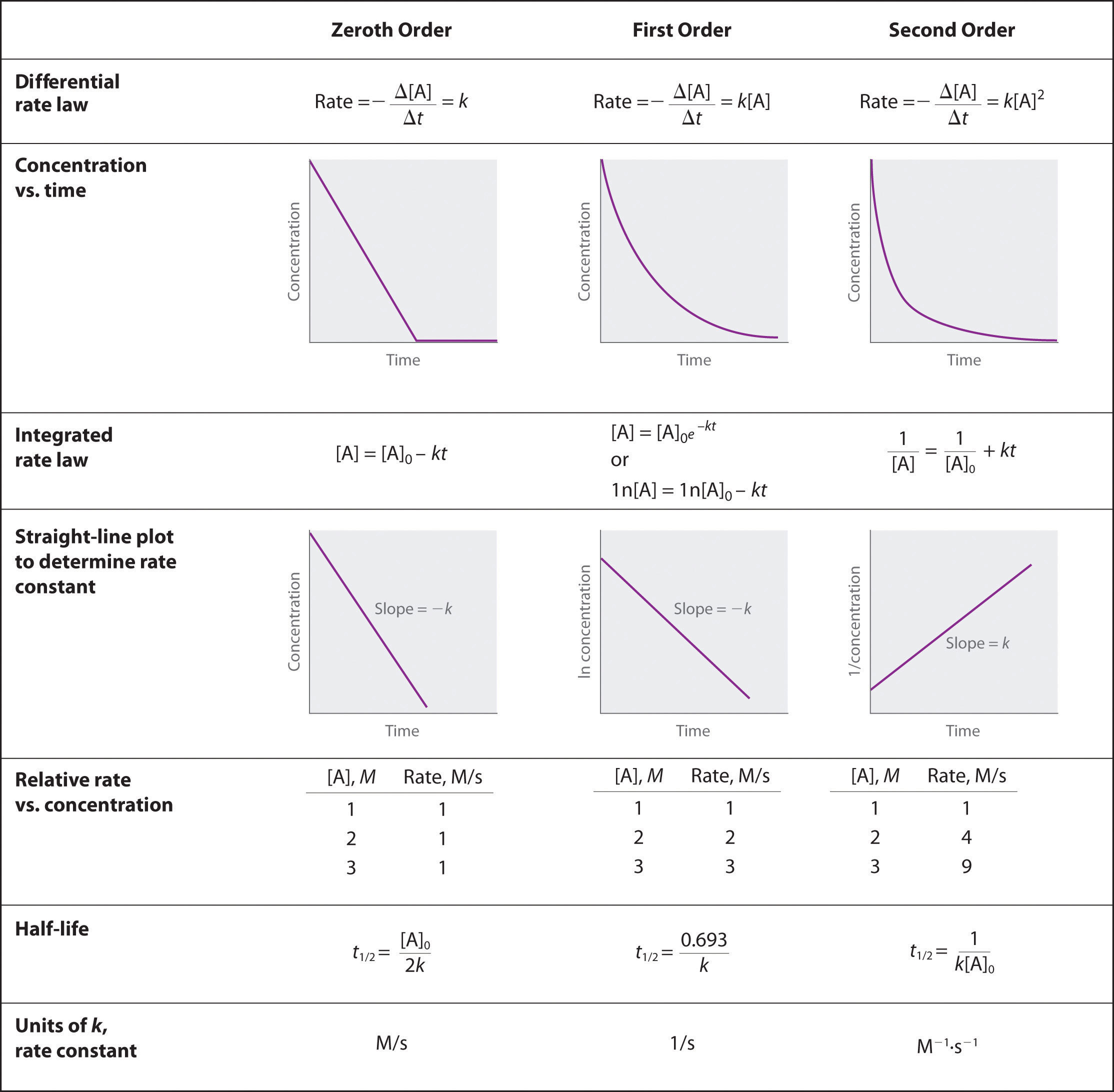
The above table summarizes the material in sections 14.4.3.and 14.4.4
Test Yourself
Homework: Section 14.5
Query \(\PageIndex{1}\)
Query \(\PageIndex{2}\)
(Note, there are around 30 worked problems in the homework, and you need to be able to do them)
Worksheet and Key:
Robert E. Belford (University of Arkansas Little Rock; Department of Chemistry). The breadth, depth and veracity of this work is the responsibility of Robert E. Belford, rebelford@ualr.edu. You should contact him if you have any concerns. This material has both original contributions, and content built upon prior contributions of the LibreTexts Community and other resources, including but not limited to:
- Liliane Poirot
- d


