6: Acid-Base Equilibria Part 1

Learning Objectives

Goals: 

• Understand that parts of an acid-base titration
• be able to determine the K_a or K_b from pH data associated with the titration of a weak acid or base
• be able to determine the molar mass of a solid monoprotic acid from titration data
• be able to calculate K_a1 and K_a2 for a polyprotic acid

By the end of this lab, students should be able to:

• design, develop and perform acid base titrations

Prior knowledge:

• Stoichiometry of Acid-Base Titrations in quantitative analysis (section 4.7.2)
• pH and pOH  (section 16.2)
• pH of Weak Acids and Bases (section 16.3, 16.5.4 and 16.5.5)
• pH of salts (sections 16.4, 16.5.6 and 16.5.7)
• buffers (section 17.2)

 

Preface

In the first semester general chemistry course the concepts of limiting and excess reagents (section 4.2) and percent yield (section 4.3) were introduced. In this treatment chemical reactions were considered to be unidirectional (Reactants → Products) and the percent yield was based on the complete consumption of the limiting reagent. It was pointed out the the percent yield would often be less than 100% and the following four reasons were discussed (section 4.3).

1. Kinetics (reaction not over, too slow to observe)
2. Equilibria (reactions are bidirectional Reactants ⇌ Products)
3. Competing/Parallel Reactions (other reactions may be consuming reactants)
4. Intermediates (the mechanism may result in intermediates that may incompletely react (equilibria) or undergo other (competing) reactions.

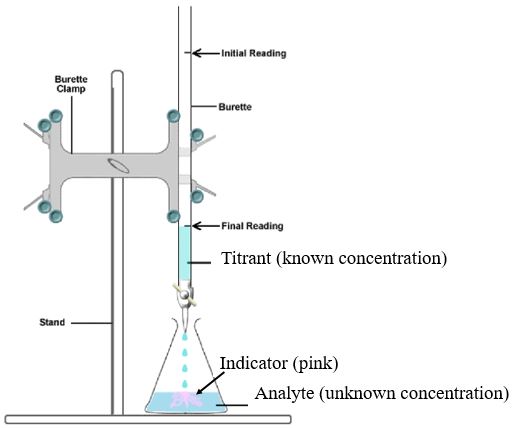
The next several labs will involve laboratory techniques that take into account the equilibrium chemistry associated with the stoichiometry of chemical reactions. The first will involve titrations of acid base reactions that may include the equilibria of weak acids or bases and the second will deal with the formation of complex ions.  The stoichiometery of acid base titrations were introduced in the first semester (section 4.7) as an analytical technique to determine the concentration of an unknown (the analyte) by measuring the quantity of a known standard (the titrant) that would react with it in stoichiometric proportions.  The analyte may be strong or weak, but the titrant must be strong and typically is monoprotic. In those experiments a pH indicator was used that changed color at the end point, which if correctly chosen was when the reactants were combined in stoichiometric proportions and thus the same as the equivalence point.  For a monoprotic acid titrated by a monoprotic base the equivalence point is when the reagents are combined in storichiometric proportions and the acid has been converted to its conjugate base.  The pH at this point is defined by the K_b', the equilibrium constant of the acid's conjugate base.  Figure \(\PageIndex{1}\) shows the basic setup for a titration using an indicator.

Figure \(\PageIndex{1}\): Setup for determining the concentration of an unknown through a titration. 

To understand the equilibrium chemistry pH titrations will involve a pH probe emerged into the analyte to measure the pH as a function of the volume titrant added and generate a titration curve, which is a plot of the pH as a function of the volume of titrant added.  The pH is the dependent variable and the volume titrant added is the independent variable. Figure \(\PageIndex{2}\) shows two titrations curves, that of a strong acid being titrated by a strong base, and that of a strong base being titrated by a strong acid.

Figure \(\PageIndex{2}\): Titration curves for (a) strong acid with strong base and (b) strong base with strong acid.

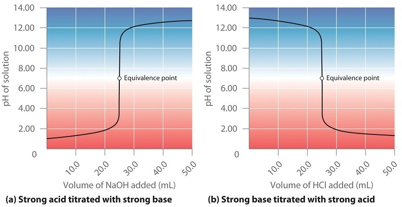
When the volume of the titrant is zero you have pure analyte and at the equivalence point the moles titrant are stoichiometrically related to the moles analyte, which has been neutralized into its conjugate. In the region between the pure analyte and the equivalence point the analyte is the excess reagent and after the equivalence point the titrant is the excess reagent. If the titration is of a strong acid and strong base (K>>1) the reaction can be considered to go to completion and calculations can be based on the complete consumption of the limiting reagent, as was done in the first semester.  If one of the analytes is weak (K<<1) the reaction does not go to completion and the equilibrium constant needs to be taken into account (sections 16.5.4 & 16.5.5). Note, if the analyte is a polyprotic (section 17.3.6) you will have multiple equivalent points and these will be distinct if the difference in successive K values are greater than 1000 (section 16.5.8). The last experiment of this lab will involve the virtual titration of a polyprotic acid

Titration of a weak monoprotic acid with a strong base.

Figure \(\PageIndex{3}\) shows the four "regions" of the titration curve for the titration of a weak acid with a strong base. It should be noted that region two is a buffer because there is excess acid (analyte) and so only part of it been neutralized by the base and converted to it's salt (the acid's conjugate base). This is one of the two ways to make a buffer (see section 17.2.3).

Weak Acid + Strong Base -> Salt +Water

where the salt is the conjugate base of the acid.

The four parts of the titration curve are described below and you should look to the approriate text section to see how they are treated.

1. Pure Acid (0 ml of base is added, section 17.3.2.1)
2. Excess acid (you have not added enough base to neutralize all of it and so have a buffer of the weak acid and it's salt, section 17.3.2.2)
   • K_a can be calculated from the pH at half equivalence (section 17.3.2.2.1)
3. Equivalence Point (the acid and base are in stoichiometric proportions and you effectively have the salt of the weak acid, section 17.3.2.3)
   • The acid and base are in 1 to 1 ratio at the equivalence point and so the initial moles acid can be calculated from the moles base at this point (n_A=n_B and n_B=M_BV_B)
     • If the acid was a solution you can determine its molarity from he volume titrated.
     • If the acid was a solid you can determine its molar mass from the mass titrated.
4. Excess Base (you have added more base than there was acid, section 17.3.2.4)

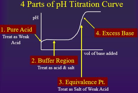
Figure  \(\PageIndex{3}\): Four parts of the titration curve for a weak acid being titrated with a strong base. Notice that two parts are points (1 & 3) and two parts are regions (2 & 4).

Be sure to go over the four parts of the titration curve in section 17.3.2 as that material is not being repeated here.  If you are titrating a weak base with a strong acid you should go over section 17.3.4

pH Probes

In this experiment we will use a Ph probe, which is an electronic device that measures the pH. These are very common and they should always be checked against standard solutions of known pH and calibrated if they read incorrectly. The pH probe is an electrochemical cell and we will cover these in chapter 19, sections 19.3-19.5 and 19.7. The following YouTube from Oxford Press does an excellent job of describing how a pH probe works.  It is imperative that you test your probe in a buffer to be sure it is reading accurately and if it is not, you will need to calibrate it.

Video \(\PageIndex{1}\) 2:30 YouTuve describing the operation of a pH probe developed by Oxford University Press (https://youtu.be/aIn4D2QXUy4).

The pH reading is not accurate until the probe stabilizes, so when you change the pH you need to wait until the reading becomes steady before recording the value.

 

Remote Labs

Due to COVID 19 you will not be able to run a titration yourself and so we are going to run two types of experiments.  The first is an IOT-enhanced lab where your instructor will run the experiment and stream the data to you over the web in real time, and the second will involve a virtual lab developed by David Yaron at Carnegie Mellon University.

Internet of Things (IOT)

The Internet Of Things (IOT) is the digital networking of physical objects and this class will use a Raspberry Pi microcomputer to stream data to a Google Sheet in real time.  Figure \(\PageIndex{4}\) shows a pH probe connected to a Raspberry Pi that is being run in desktop mode.  Students will be able to remotely access the Raspberry Pi by using the free VNC Viewer software, or by being giving control of their instructor's computer through Zoom. How this is done will vary from instructor to instructor.

Figure \(\PageIndex{4}\): Copy and Paste Caption here. (Belford, cc 3.0)

Figure  \(\PageIndex{5}\) shows the schema for how the class will be run.  The Raspberry Pi will stream data to a special Google sheet through an API (Application Program Interface) that allows the sheet to capture the data over the internet in real time.  The instructor or a student will type into a Python program on the pi the total volume of base added (independent variable) and then press enter, at which time the Pi will send that data along with the pH (dependent variable) to the API sheet.  The students and instructor's Google Sheets will then grab that data and display it in a tab called "data".  The instructor will then add some more titrant, and once the pH reading stabilizes they will type in the new volume, submit it, and repeat the cycle until they have at least 5 mL in the excess base region.

 

Figure \(\PageIndex{5}\): Schematic of how an IOT-enhanced lab is performed (Belford; cc 3.0)

 

The Experiment

Safety

In this experiment we will titrate acetic acid with sodium hydroxide. Sodium hydroxide can cause chemical burns and blindness. Eye protection is required and the following image shows the damage 4 M sodium hydroxide can cause.  By following proper procedures and using proper PPE (Personal Protective Equipment) the risk to damage can be reduced to near zero. There are two primary factors that determine the extent of injury due to exposure to corrosive chemicals like NaOH, the concentration of the chemical and the time of contact (exposure to the chemical).  For this reason we do not perform titrations with concentrated acids and bases, but dilute ones.  If you ever have an acid or base spill you need to immediately inform your instructor, who will clean it up or instruct you on what to do.  If you spill it on your body you should immediately wash it off with copious amounts of water.

Figure \(\PageIndex{6}\): Left image, chemical burn due to 4M NaOH, eye protection is mandatory. (Prof. N. Schrage, Dept. of Ophthalmology, Cologne Merheim, RWTH Aachen, posted with permission for educational purposes only). Right image, chemical burn 44 hours after exposure to <10% by weight NaOH solution (Balsiuz, Wikimedia Commons)

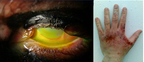
The best protection to prevent injury is to minimize risk and thus students are required to abide by safety protocols by wearing proper PPE such as chemical splash goggles, closed top shoes and pants. In the event of an accident there is an eye wash and safety shower.  If you spill a corrosive chemical on your clothes the instructor will empty the room of all students and you must remove the exposed clothes when you take the shower as it is imperative that you reduce the time  and amount of contact to the hazardous chemical. 

Figure \(\PageIndex{7}\): Eye Wash and Safety Shower in general chemistry lab at UALR (Belford, CC 3.0)

It should also be noted that some acids, like HydroFluoric acid (a weak acid) can be fatal even though there may be no visible damage until 12 to 24 hours after exposure (see this fact sheet from the CDC). The experiments we perform in the general chemistry teaching labs are designed with safety in mind and all effort is made to minimize risk, but it is imperative that student develop an understanding of proper safety protocols as they may need them long after the class is over.  In the event of an accident always alert the instructor, even if it seems to be a trivial spill, and always seek professional medical advice if you have an accident outside of the lab or university.

Exercise \(\PageIndex{1}\)

A student spills NaOH on their skin, should they neutralize it with an acid?

Answer

No!  They should rinse it with copious amounts of water.  Acid-Base reactions are exothermic and can cause heat that can do further damage, and there is no reason to think the acid will come to contact with the base before it contacts your flesh, and in effect compounds the problem.  You can neutralize a solution of a base like sodium hydroxide by adding HCl to it, and if they are in stoichiometric proportions create sodium chloride. But a skin burn is completely different and you should pour copious amounts of water on it, and seek expert advice.

In your Google Doc you will need to look up and submit a link to the SDS of all reagents and link to the PubChem LCSS. Although these resources of are of great value, they do not substitute for professional medical advice and in the event that you ever have a chemical spill you need to contact a qualified medical service to seek help.

 

Experimental Design

The goal is to identify the equivalence point and the pH at half equivalence.  By knowing the equivalence point one can determine moles analyte (Acetic Acid) that was titrated, and by knowing the pH at half equivalence one can determine the acid dissociation constant (K_a). 

Exploratory Run

Before doing a titration with a pH probe you should do an exploratory run with a pH indicator. You want to choose an indicator that changes color at a pH that is equal to the pH of the salt of the weak acid formed at the equivalence point. The following graph provides the pH that common indicators change at.

Figure \(\PageIndex{8}\): Color changes for some common pH indicators as a function of pH. Note, some diprotic indicators have different colors for the acidic, acid salt, and salt forms.

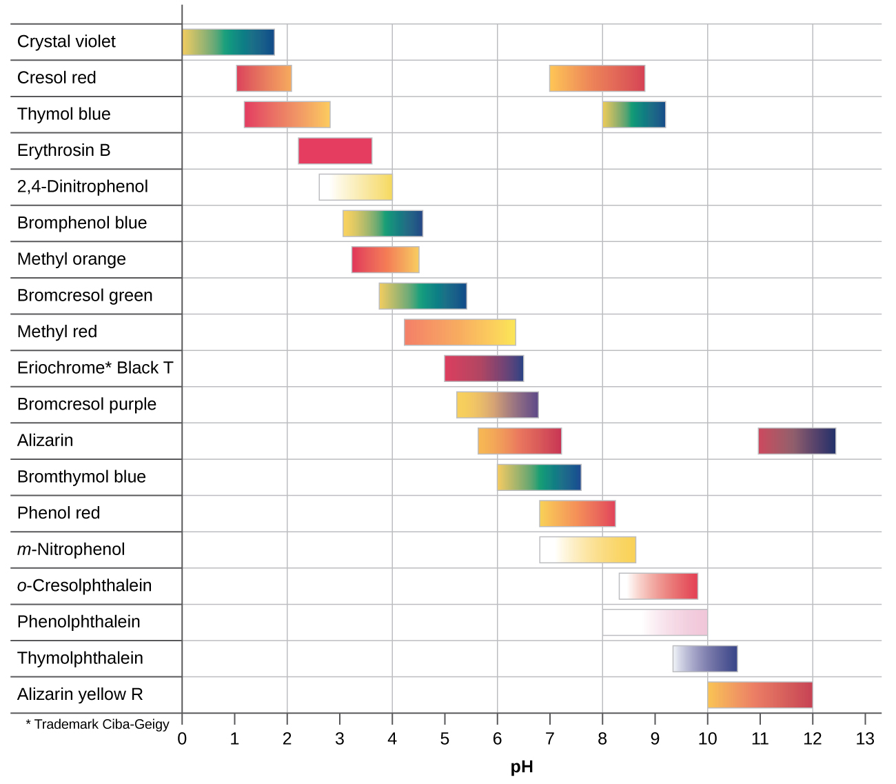
Acetic Acid has a K_a of 1.8x10^-5 and so the K_b' of acetate is \(\frac{10^{-14}}{1.8x10^{-5}}=5.55x10^{-10}\) and according to equation 17.3.10 a 0.05M solution of Acetate would have a pH of 8.72.

\[[OH^-]=\sqrt{\left (\frac{K_w}{K_b'} \right )[B]_i}  \; \\ \; \\ [OH^-]=\sqrt{\left (\frac{10^{-14}}{1.8x10^{-5}} \right )(0.05M)} = 5.27x10^{-6}\]

So the pOH of a 0.05M solution of Acetate is -log(5.27x10^-6 = 5.27 and the pH = 14-5.27 = 8.72.  This would make phenolphthalein a good indicator for the titration of acetic acid.

In the next section we will look at the parts of the titration curve and see that a lot of data is needed around the equivalence point, where you should make measurements dropwise, and a little at half equivalence, and during the rest of the buffer region one can make a measurement every couple of milliliters or so, and should not spend an excessive amount of time.

 

Identification of the equivalence point

If one looks at a titration curve (\(\PageIndex{9}\)) they will note that the slope of the line starts of fairly flat (buffer region) and then starts to increase as the equivalence point is approached and then it starts to flatten out again after equivalence, becoming fairly flat again in the excess base regions. The slope of the line is actually the derivative \(\left ( lim \;\Delta V \to 0 \;  \frac{\Delta pH}{\Delta V} \right )\) and the equivalence point can be identified when this changes from an increasing value to a decreasing value. That is, when the rate of change of the slope goes from a positive (increasing value) to a negative (decreasing value) and this is known as the inflection point, which can be obtained by observing when the second derivitive \(\left ( lim \;\Delta V \to 0 \;  \frac{\Delta^2 pH}{\Delta V^2} \right )\) goes to zero.

Figure \(\PageIndex{9}\): pH Tiration curve with first and second derivative plots. (Belford cc 0)

What should be noticed from figure \(\PageIndex{9}\) is that you need a lot of data around the equivalence point (green oblongs) and a little data at half equivalence (red circle). So after you have done your exploratory run you want to design your experiment so you get data where you need it, and do not waste time getting lots of data where you do not need it.  Be sure to collect data 5 mL past the equivalence point.

 

Determination of K_a

K_a can be determined by reading the pH at half equivalence (when half of the acid has been neutralized and converted to its salt).  This is in the buffer region and uses the Henderson Hasselbach equation

\[pH=pK_a+\log \dfrac{[A^-]}{HA}\]

Since at half equivalence [HA]=[A^-] pH = pK_a , at half equivalence

so 

\[K_a =10^{-pH\text{, at half equivalence}} \]

So you find the equivalent point on the titration curve and read the value of the curve at half of that volume.  For this reason you need to collect data half way along the curve (red circle).

 

Determining the moles acid (analyte)

This is really a gen chem 1 stoichiometry problem, and at the equivalence point the moles of base added equals the moles of protons transferred, which is the moles of acid for a monoprotic acid.  As we shall see, polyprotic acids will have more than one equivalence point as they can donate more than one proton, and each of the protons has its own K_a.

Actual Experiment

The instructor will set up and run the experiment like a real-time demonstration, but stream it to your Google Sheet in real time.  The following image shows the initial setup.

Figure \(\PageIndex{10}\): Copy and Paste Caption here. (Copyright; author via source)

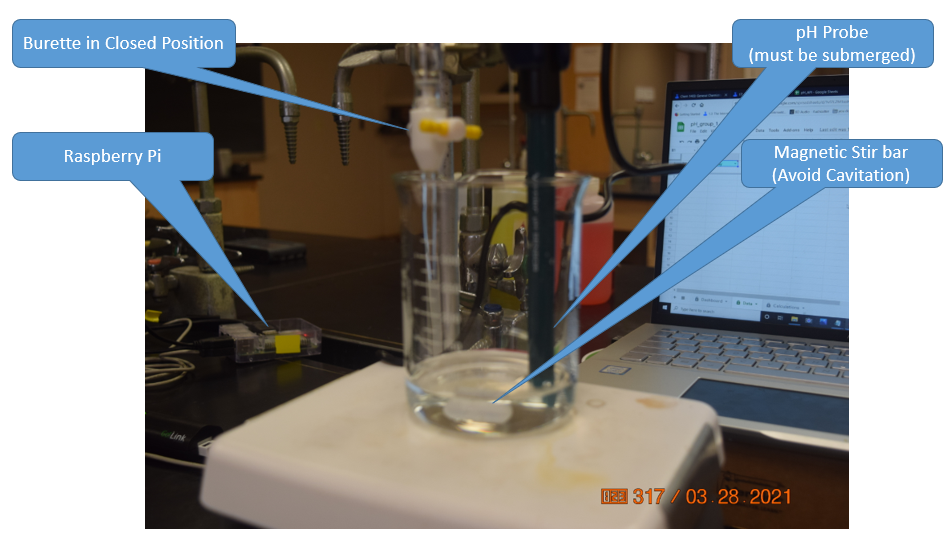
The magnetic stir bar is used to make sure there are no concentration gradients. Be sure to add enough water to submerge the pH probe and take the dilution effect of this water into account when determining the initial concentration of the acid. It takes a while for the pH meter to stabilize and so we will run a second program to read the pH, and when it reaches a constant value it will be entered to the Google Sheet.

 

Your instructor will run the actual experiment and stream the data to your Google Sheet.  There will be two programs running on the Raspberry Pi

Figure \(\PageIndex{11}\): The Raspberry Pi Desktop is being overlaid a Google sheet by the VNC Vierwer in this screen capture.  There are two Python programs being run, one in command line and one in the Thonny IDE (Interactive Development Environment).  The white text on the black background is the program being run in command line and every 10 seconds it displays the current pH.  The program in Thonny is running a program "PH_Vernier_sheets_append", which allows a user to enter the volume and when the hit <Enter> it takes that volume and pH and appends it to the Google Sheet in the foreground. (Belford, cc 3.0)

 One of the problems students have is that they often do not wait for the pH reading to stabilze between successive readings, and that is why we have the second program running in the command line.

 

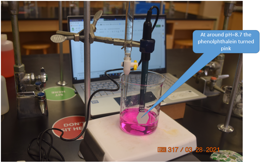Figure \(\PageIndex{12}\): At around pH=8.7 the indicator turned pink, and the titration was continued for another 5 mL into the excess base region. As there was only one person in the lab we ignored the COVID-19 seating assignments, but if students attend labs they need to sit where the green stickers are (Belford, cc 3.0)

 

Google Workbook

Workbooks are a way of organizing your google sheet. A workbook has a tab for each section of data and a dashboard to summarize the results. This helps to be able to understand your data at a glance.

Your instructor will give you access to your groups workbook.

Dashboard

The first tab of the google sheet is your dashboard. This is summarizes your results all in one place.

Only the boxes with a blue background can be edited. Fill out the sections for Group #, Experiment #, Lab Section, Date, and members names. After completing the lab fill out the results and paste charts into the titled boxes.

Data Tab

You can navigate to the data tab by clicking the tab on the bottom of your screen.

In cell B1 there is a drop down arrow, use this to select your lab section (9H1-9H6)

Now as the instructor performs the experiment you will get a live feed of the data

If you have a #REF error follow the steps in Figure 1 to resolve it

Figure \(\PageIndex{13}\): If you get a #ref error click on the cell, it will say you need to connect the sheets, click allow access to fix it (Poirot)

Calculations

Titration Curve

Copy the data from the data tab and paste it into columns A and B using ctrl+shift+v (this pastes values only)

Plot the titration curve by making a chart of pH vs. mL NaOH. Resize the chart by clicking and dragging one of the corners to make it fit in the box for titration curve.

First Derivative

The first derivative curve is simply a plot of the slope of the titration curve versus the volume of base added.

The equivalence point volume will correspond to the highest point in the first derivative plot.

\[ \frac{\Delta  pH}{\Delta  V}=\frac{pH_{2}-pH_{1}}{V_{2}-V_{1}} \]

This is the slope between two data points and so we relate it to the average value of those two data points. All of this to say we will take the average of the two volumes to use as our x cordinate.

Figure \(\PageIndex{14}\): example of the formula for the First Derivative (Poirot)

Repeat this formula for all the data (note you should end with one less data point than the original)

Make a chart for your First Derivative plot of \(\frac{\Delta pH}{\Delta V} \) vs. avg V

Second Derivative

The second derivative repeats the same formula using the results from the first derivative.

\[\frac{\Delta(\frac{\Delta  pH}{\Delta  V})}{\Delta V}=\frac{pH_{deriv2}-pH_{deriv1}}{V_{avg2}-V_{avg1}}=\frac{\frac{\Delta^{2}  pH}{\Delta  V^{2}}}{\Delta V}\]

Just like for the first derivative, this is the slope between the two data pointsm so we will relate it to the average value of the two data points. Basically meaning we will take the average of the two Volumes from the first derivative as our x axis

Figure \(\PageIndex{15}\): example of the formula for the SeondDerivative (Poirot)

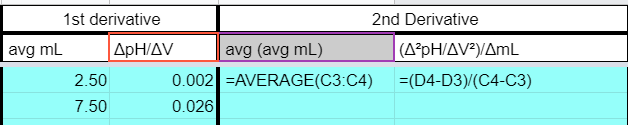
Repeat this for all the data points, just like before you should end up with one less point than the first derivative, and two less than the original data.

Make a chart for your second derivative plot of \(\frac{\frac{\Delta^{2}  pH}{\Delta  V^{2}}}{\Delta V}\) vs avg (avg V)

Charts Basics

If you are unfamiliar with using charts in google sheets follow these tutorials.

Video \(\PageIndex{2}\): 3:49 video developed by Liliane Poirot on inserting and editing a chart (https://youtu.be/201tlRiHmw0)

Insert a Chart

To insert a chart first highlight the cells you want in your chart

If you highlight the columns this will use all data in those columns which is useful if you add more later

Next click Insert then Chart

Edit a Chart

To edit a chart click the three dots in the right hand corner of the chart, this will open the chart tool bar to the right.

Setup lets you choose the type of chart and the other basic set up for the chart. Figure 1 below explains the different options in the setup menu.

Figure \(\PageIndex{16}\): Labeled Chart Editor Toolbar (Poirot)

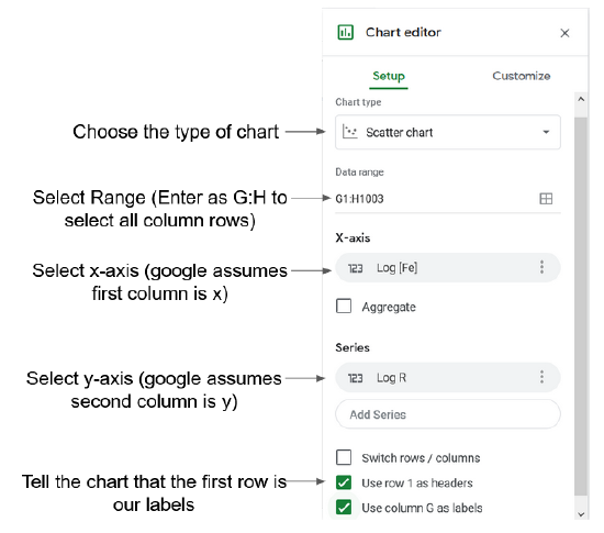
You can also customize a chart using the customize tab. This lets you change the look of a chart.

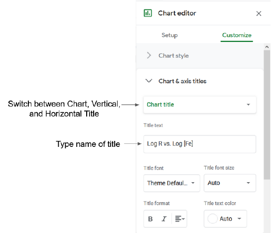
Chart & Axis Titles

You can change the title of the chart or the x and y axis of a chart. If you have Use row 1 as headers checked the sheet should automatically use your first row as the title for the axis.

To change the title you can go to the chart toolbar then customize and select Chart & Axis Titles.

You can switch between the Chart Title, the Horizontal Axis (x), and the Vertical Axis (y) and change the title text.

Alternatively you can change the text by double clicking on the title you want to change

Figure \(\PageIndex{17}\):Changing the title of a chart or axis. (Poirot)