
17.3: Acid-Base Titrations
- Page ID
- 60763

\( \newcommand{\vecs}[1]{\overset { \scriptstyle \rightharpoonup} {\mathbf{#1}} } \)
\( \newcommand{\vecd}[1]{\overset{-\!-\!\rightharpoonup}{\vphantom{a}\smash {#1}}} \)
\( \newcommand{\dsum}{\displaystyle\sum\limits} \)
\( \newcommand{\dint}{\displaystyle\int\limits} \)
\( \newcommand{\dlim}{\displaystyle\lim\limits} \)
\( \newcommand{\id}{\mathrm{id}}\) \( \newcommand{\Span}{\mathrm{span}}\)
( \newcommand{\kernel}{\mathrm{null}\,}\) \( \newcommand{\range}{\mathrm{range}\,}\)
\( \newcommand{\RealPart}{\mathrm{Re}}\) \( \newcommand{\ImaginaryPart}{\mathrm{Im}}\)
\( \newcommand{\Argument}{\mathrm{Arg}}\) \( \newcommand{\norm}[1]{\| #1 \|}\)
\( \newcommand{\inner}[2]{\langle #1, #2 \rangle}\)
\( \newcommand{\Span}{\mathrm{span}}\)
\( \newcommand{\id}{\mathrm{id}}\)
\( \newcommand{\Span}{\mathrm{span}}\)
\( \newcommand{\kernel}{\mathrm{null}\,}\)
\( \newcommand{\range}{\mathrm{range}\,}\)
\( \newcommand{\RealPart}{\mathrm{Re}}\)
\( \newcommand{\ImaginaryPart}{\mathrm{Im}}\)
\( \newcommand{\Argument}{\mathrm{Arg}}\)
\( \newcommand{\norm}[1]{\| #1 \|}\)
\( \newcommand{\inner}[2]{\langle #1, #2 \rangle}\)
\( \newcommand{\Span}{\mathrm{span}}\) \( \newcommand{\AA}{\unicode[.8,0]{x212B}}\)
\( \newcommand{\vectorA}[1]{\vec{#1}} % arrow\)
\( \newcommand{\vectorAt}[1]{\vec{\text{#1}}} % arrow\)
\( \newcommand{\vectorB}[1]{\overset { \scriptstyle \rightharpoonup} {\mathbf{#1}} } \)
\( \newcommand{\vectorC}[1]{\textbf{#1}} \)
\( \newcommand{\vectorD}[1]{\overrightarrow{#1}} \)
\( \newcommand{\vectorDt}[1]{\overrightarrow{\text{#1}}} \)
\( \newcommand{\vectE}[1]{\overset{-\!-\!\rightharpoonup}{\vphantom{a}\smash{\mathbf {#1}}}} \)
\( \newcommand{\vecs}[1]{\overset { \scriptstyle \rightharpoonup} {\mathbf{#1}} } \)
\(\newcommand{\longvect}{\overrightarrow}\)
\( \newcommand{\vecd}[1]{\overset{-\!-\!\rightharpoonup}{\vphantom{a}\smash {#1}}} \)
\(\newcommand{\avec}{\mathbf a}\) \(\newcommand{\bvec}{\mathbf b}\) \(\newcommand{\cvec}{\mathbf c}\) \(\newcommand{\dvec}{\mathbf d}\) \(\newcommand{\dtil}{\widetilde{\mathbf d}}\) \(\newcommand{\evec}{\mathbf e}\) \(\newcommand{\fvec}{\mathbf f}\) \(\newcommand{\nvec}{\mathbf n}\) \(\newcommand{\pvec}{\mathbf p}\) \(\newcommand{\qvec}{\mathbf q}\) \(\newcommand{\svec}{\mathbf s}\) \(\newcommand{\tvec}{\mathbf t}\) \(\newcommand{\uvec}{\mathbf u}\) \(\newcommand{\vvec}{\mathbf v}\) \(\newcommand{\wvec}{\mathbf w}\) \(\newcommand{\xvec}{\mathbf x}\) \(\newcommand{\yvec}{\mathbf y}\) \(\newcommand{\zvec}{\mathbf z}\) \(\newcommand{\rvec}{\mathbf r}\) \(\newcommand{\mvec}{\mathbf m}\) \(\newcommand{\zerovec}{\mathbf 0}\) \(\newcommand{\onevec}{\mathbf 1}\) \(\newcommand{\real}{\mathbb R}\) \(\newcommand{\twovec}[2]{\left[\begin{array}{r}#1 \\ #2 \end{array}\right]}\) \(\newcommand{\ctwovec}[2]{\left[\begin{array}{c}#1 \\ #2 \end{array}\right]}\) \(\newcommand{\threevec}[3]{\left[\begin{array}{r}#1 \\ #2 \\ #3 \end{array}\right]}\) \(\newcommand{\cthreevec}[3]{\left[\begin{array}{c}#1 \\ #2 \\ #3 \end{array}\right]}\) \(\newcommand{\fourvec}[4]{\left[\begin{array}{r}#1 \\ #2 \\ #3 \\ #4 \end{array}\right]}\) \(\newcommand{\cfourvec}[4]{\left[\begin{array}{c}#1 \\ #2 \\ #3 \\ #4 \end{array}\right]}\) \(\newcommand{\fivevec}[5]{\left[\begin{array}{r}#1 \\ #2 \\ #3 \\ #4 \\ #5 \\ \end{array}\right]}\) \(\newcommand{\cfivevec}[5]{\left[\begin{array}{c}#1 \\ #2 \\ #3 \\ #4 \\ #5 \\ \end{array}\right]}\) \(\newcommand{\mattwo}[4]{\left[\begin{array}{rr}#1 \amp #2 \\ #3 \amp #4 \\ \end{array}\right]}\) \(\newcommand{\laspan}[1]{\text{Span}\{#1\}}\) \(\newcommand{\bcal}{\cal B}\) \(\newcommand{\ccal}{\cal C}\) \(\newcommand{\scal}{\cal S}\) \(\newcommand{\wcal}{\cal W}\) \(\newcommand{\ecal}{\cal E}\) \(\newcommand{\coords}[2]{\left\{#1\right\}_{#2}}\) \(\newcommand{\gray}[1]{\color{gray}{#1}}\) \(\newcommand{\lgray}[1]{\color{lightgray}{#1}}\) \(\newcommand{\rank}{\operatorname{rank}}\) \(\newcommand{\row}{\text{Row}}\) \(\newcommand{\col}{\text{Col}}\) \(\renewcommand{\row}{\text{Row}}\) \(\newcommand{\nul}{\text{Nul}}\) \(\newcommand{\var}{\text{Var}}\) \(\newcommand{\corr}{\text{corr}}\) \(\newcommand{\len}[1]{\left|#1\right|}\) \(\newcommand{\bbar}{\overline{\bvec}}\) \(\newcommand{\bhat}{\widehat{\bvec}}\) \(\newcommand{\bperp}{\bvec^\perp}\) \(\newcommand{\xhat}{\widehat{\xvec}}\) \(\newcommand{\vhat}{\widehat{\vvec}}\) \(\newcommand{\uhat}{\widehat{\uvec}}\) \(\newcommand{\what}{\widehat{\wvec}}\) \(\newcommand{\Sighat}{\widehat{\Sigma}}\) \(\newcommand{\lt}{<}\) \(\newcommand{\gt}{>}\) \(\newcommand{\amp}{&}\) \(\definecolor{fillinmathshade}{gray}{0.9}\)Introduction
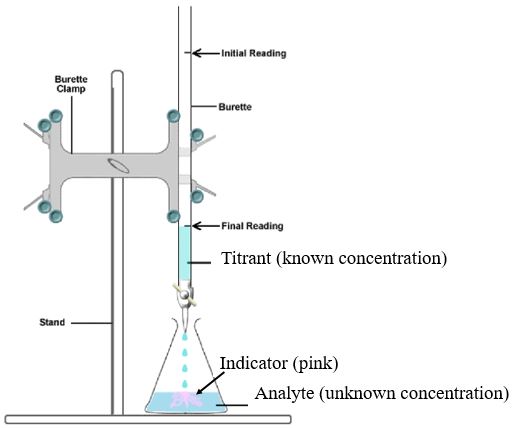
Titrations are an analytical technique most commonly used to calculate the concentration of an unknown (the analyte) with a known (the standard, or titrant). The principle is fairly simple, if you know the stoichiometry of a reaction and the quantity of one species, you can calculate the quantity of the other, the trick is to figure out when they are in stoichiometric proportions. One technique is to use an indicator, which is another substance that changes color when the reaction is completed. There are many types of titrations (acid-base, redox), they all involve a reaction where you add one reactant incrementally until they are in stoichiometric proportions, and then knowing the moles of the titrant, you can calculate the moles of the analyte. If the analyte is a solid and you measure it's mass, information on its molar mass can also be obtained.
There are two basic types of acid base titrations, indicator and potentiometric. In an indicator based titration you add another chemical that changes color at the pH equal to the equivalence point, when the acid and base are in stoichiometric proportions. In a potentiometric titration you record the pH as you add titrant, and if the analyte is a weak acid or base you can determine its \(K_a\) or \(K_b\).
Relating Titrations to Stoichiometric Equations
Relating titrations to stoichiometry and limiting reagent problems. Consider the titration of \(\ce{HCl}\) with \(\ce{NaOH}\), that is, \(\ce{HCl}\) is the analyte and \(\ce{NaOH}\) is the titrant.
\[\ce{HCl + NaOH \rightarrow NaCl + H_2O}\]
As you titrate this you have four types of stoichiometric relationships
- Initially - Pure \(\ce{HCl}\) (you have added no \(\ce{NaOH}\))
- \(\ce{HCl}\) is the excess reagent, \(\ce{NaOH}\) is the limiting reagent (you have not added enough \(\ce{NaOH}\) to react with all the \(\ce{HCl}\))
- \(\ce{HCl}\) and \(\ce{NaOH}\) are in stoichiometric proportions (you have added just enough \(\ce{NaOH}\) to neutralize the \(\ce{HCl}\), but none extra)
- \(\ce{NaOH}\) is the excess reagent and \(\ce{HCl}\) is the limiting reagent (once you have neutralized all the HCl, any more \(\ce{NaOH}\) is excess).
So the objective of the titration is to find part 3, when the acid and base are in stoichiometric proportions, and knowing the quantity of titrant at that point allows one to calculate the moles of analyte.
Running a Titration
4:50 min YouTube by RSC. Note, this is a very good video, but there was a potential mistake in that they did not flush out the bottom of the stopcock, but since this was an overshoot run, it made no difference. That is, below the stopcock fluid collects, and you should run the titrant through the burette to make sure no air bubbles get trapped.
Virtual Lab
Try your own titration with the following virtual lab
Four Basic Types of Acid-Base Titrations
Table \(\PageIndex{1}\) shows the four types of titrations, and you note that the titrant (compound in the burette that is added to the analyte) is always strong, while the analyte can be strong or weak. This is because in running a titration it is imperative that the titrant completely react, that way you can say that the moles hydronium or hydroxide added is equal to the molarity times the volume (n=MV) of the titrant. This allows you to calculate the amount of salt produced by the complete consumption of the titrant (up to the triple point). If that salt then reacts to form the acid of it's conjugate relationship, you can calculate the "initial" concentration based on the amount of titrant added.
| Type | Analyte | Titrant |
|---|---|---|
| SA/SB | Strong Acid | Strong Base |
| WA/SB | Weak Acid | Strong Base |
| SB/SA | Strong Base | Strong Acid |
| WB/SA | Weak Base | Strong Acid |
Strong Acid-Base (SA/SB & SB/SA)
We will treat both SA/SB and SB/SA calculations concurrently because these are essentially general chemistry 1 limiting reagent problems. You simple calculate the moles acid and the moles base, and base the pH on the concentration of the excess reagent. Because these reactions go to completion they do not form buffers.
Initially, before any titrant is added, the pH is that of a pure acid or pure base, and the hydronium/hydroxide ion concentration is that of the pure acid or pure base.
Before Equivalence point
The Analyte is the Excess Reagent, and so you need to calculate the moles excess analyte and divide by the total volume, and from that answer the question, which is usually, what is the pH.
\[\large{[Analyte]_{excess} = \frac{(n_{analyte}-n_{titrant})}{V_T}=\frac{(M_{analyte}V_{analyte})-(M_{titrant}V_{titrant})}{V_{analyte}+V_{titrant}}}\]
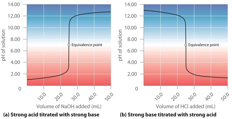
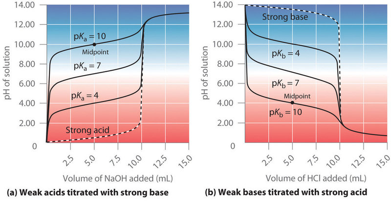
Note, in Figure\(\PageIndex{2a}\), the pH < 7 because the analyte is an acid and you have not neutralized it all, while in Figure\(\PageIndex{2b}\) the pH > 7 because the analyte is a base, and you have not neutralized it all
Equivalence Point
At the equivalence point moles acid = moles base and the pH = 7 because the salt of a strong acid and a strong base is neutral (the ions do not protonate or remove a proton from water)
After Equivalence Point
The Titrant is the Excess Reagent, and so you need to calulate the moles excess titrant and divide by the total volume, and from that answer the question, which is usually, what is the pH.
\[\begin{align} [Titrant]_{excess} &= \frac{(n_{titrant}-n_{analyte})}{V_T} \\[5pt] &=\frac{(M_{titrant}V_{titrant})-(M_{analyte}V_{analyte})}{V_{analyte}+V_{titrant}} \end{align} \]
Note, in Figure\(\PageIndex{2a}\), the pH > 7 because the titrant is a base and you have added more than was required to neutralize the analyte (acid), while in Figure\(\PageIndex{2b}\) the pH < 7 because the titrant is an acid and you have added more than was required to neutralize all the analyte (base).
Weak Acid with Strong Base
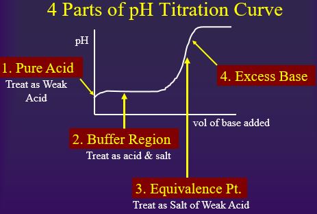
There are four parts to the titration curve of a weak acid (analyte) with a strong base(titrant).
- Initial pH (pH of a weak acid)
- Buffer Equation (Henderson Hasselbach Eq.)
- Equivalence Point (salt of weak acid)
- Excess Base (pH based on concentration of excess titrant)
NOTE: A typical question is like: What is the pH when Xml (Vb) of Y molar (Mb) strong base has been added to Q ml ((Va) of R molar (Ma) weak acid. The first step is to figure out what region of the titration curve you are in, and then solve the problem. This can be done through the relationship na = nb (moles acid = moles base), which for liquids is MaVa = MbVb. Note, this even works for polyprotic acids, that will have more than one equivalence point (see below).
Pure Acid
Treat as a weak acid (section 16.5.4.2) \[\large{pH=-\log\sqrt{K_{a}[HA]_{i}}}\]
Buffer Region
In Section 17.2.3 it was shown that one way to make a buffer is to partially neutralize and acid and so in the buffer region we can use the Henderson Hasslebach equation.
\[pH=pK_a+\log \dfrac{[A^-]}{HA}\]
If we know the volume of base to reach equivalence (Veq), we can express the ratio \(\dfrac{[A^-]}{HA}\) as the ratio of the volume of base added at any point (Vb) to the volume of remaining base that would need to be added to completely neutralize the acid (\(V_{eq} - V_b\)), or
\[\dfrac{[V_b]}{V_{eq}-V_b}.\]
So
\[\large{\textcolor{red}{pH_{\text{at point b}}=pK_a+\log \dfrac{[V_b]}{V_{eq}-V_b}}} \label{17.3.7}\]
Equation \ref{17.3.7} not only simplifies the calculation, but allows you to determine the pH of a buffer in a titration even if you do not know the concentration of the acid or the base, as long as you know the volume of base required to neutralize the acid.. The derivation of this simplification is described in the following YouTube.
Half Equivalence
In section 17.2.5 we discussed buffer pH and that the \(pH=pK_a\) if \([HA]=[A^-]\). In a titration this is known as half equivalence or half titer, which is the volume required to titrate off half of the titratable protons (of a monoprotic acid, or the first proton of a polyprotic acid). That is, at half equivalence, \(V_b=\frac{V_{eq}}{2}\).
\[\begin{align} \large{\textcolor{red}{pH_{\text{at half titer}}}} &=pK_a+\log \dfrac{[V_b]}{V_{eq}-V_b} \nonumber \\[5pt] &=pK_a+\log\frac{\frac{V_{eq}}{2}}{V_{eq}-\frac{V_{eq}}{2}} \nonumber \\[5pt] &=pK_a + \log\frac{\frac{V_{eq}}{2}}{\frac{V_{eq}}{2}} \nonumber \\[5pt] &= pK_a + \log(1) \nonumber \\[5pt] &= pK_a+0 \nonumber \\[5pt] & \large{\textcolor{red}{=pK_a}} \end{align}\]
Why is this important? This means that if you know the concentration of an acid, you can calculate its \(pK_a\) by neutralizing half of it, and then reading the pH. If you do not know its concentration, you can titrate it, find how much base it took to neutralize it (the equivalence point), and then add half of that amount of base to another sample of the same volume of acid, and the pH is its pKa.
Virtual Lab \(\PageIndex{1}\)
With just one measurement, calculate the room temperature \(K_a\) for hydrofluoric acid using the virtual lab below.
- Activate Virtual Lab
-
Note: The virtual lab uses thermodynamic equations to calculate equilibrium conditions and operates at an ambient temperature of °C. You can rightclick on a flask and adjust its temperature directly, and you can also isolate it from the surroundings. The equilibrium constant is a function of temperature, and so you need to adjust it to 25 °C to get the correct answer, which should be \(6.61 \times 10^{-4}\).
There is a short animation on how to use the virtual lab on the UALR lab page in LibreText and additional material is available at the ChemCollective.
The Chemcollective Virtual laboratory was developed by Professor David Yaron's research group at Carnegie Mellon University.
Exercise \(\PageIndex{2}\)
What is the pH of an acetic acid solution after 20 mL of an NaOH was added if the equivalence point required 50 ml on NaOH?
- Answer
-
Since it took 50 ml to neutralize, we can easily see that 25 ml would have neutralized half of it, and at 20 ml we have neutralized \(\frac{20}{50}\) or 2/5, and have not neutralized \(\frac{50-20}{50}\) or 3/5. The fraction neutralized has been converted to the salt, and the fraction remaining is still a weak acid, so pH=pKa+log2/3, or to do it the long way:
\[\begin{align*} pH &=pK_a + \log \frac{[A^-]}{[HA]} \\[5pt] &=pK_a + \log\frac{V_b}{V_e-V_b} \\[5pt] &= -\log1.75 \times 10^{-5}+\log \frac{20}{50-20} \\[5pt] &= 4.76+(-0.40)\\[5pt] &=4.36 \end{align*}\]
This makes sense, because you have not reached half equivalence, where the \(pH = pK_a\) .
Equivalence Point
At the equivalence point the weak acid is in stoichiometric proportions to the strong base, and so it is completely converted to its salt, meaning you have the salt of a weak acid (review section 16.5.6).
\[[OH^-]=\sqrt{\left (\frac{K_w}{K_a} \right )[A^-]_i} \]
At the equivalence point moles HAinitial = moles Base added , so \(M_AV_{A,initial}=M_BV_{B.equivalence}\), which is the moles A- created, because all the HA has been converted to A-.
As you added the base to the weak acid you did two things
- Neutralized the Acid
- Diluted the Acid
Taking this into account and noting that the total volume is the volume of the initial acid \(V_{A,i}\) and the base added \(V_{B,e}\) to neutralize it
\[[OH^-]=\sqrt{\frac{K_w}{K_a}\left ( \frac{M_AV_{A,i}}{V_T} \right )} =\sqrt{\frac{K_w}{K_a}\left ( \frac{M_AV_{A,i}}{V_{A,i}+V_{B,e}} \right )}\]
or, since the definition of the equivalence point is moles HAinitial = moles base added, this can also be expressed in the molarity of the base.
\[[OH^-]=\sqrt{\frac{K_w}{K_a}\left ( \frac{M_BV_{B,e}}{V_{A,i}+V_{B,e}} \right )} \]
It does not matter which form of the above equations you use
\[\large{\textcolor{red}{pOH=-\log\sqrt{\frac{K_w}{K_a}\left ( \frac{M_BV_{B,e}}{V_{A,i}+V_{B,e}} \right )}}} \]
(convert to pH if needed)
Excess Base Region
In the excess base region you have added more strong base than there was weak acid and so this is a limiting reagent problem, and since all the strong base converts to hydroxide, you simply need to find the excess moles strong base and divide by the total concentration to get the hydroxide concentration
\[[OH^-] =\frac{n_{OH^{-},(excess)}}{V_T} =\frac{M_BV_B-M_BV_{eq}}{V_B+V_{A,i)}} \nonumber\]
\[\large{[OH^-] = \frac{M_B\left (V_B-V_{eq} \right )}{V_B+V_{A,i)}}}\]
(convert to pH if needed)
Titration Problems
General Strategy
Find out what part of the curve you are in, and then use the appropriate equation. If you have not added base Vb = 0, it is trivial and you are solving the pH for a weak acid. If you have added base, (Vb) there are three possibilities
- Vb < Vb.eq : Buffer region, base is the limiting reagent and there is un-neutralized weak acid.
- Vb = Vb,eq : Equivalence point, base and weak acid are in stoichiometric proportions and the weak acid has been converted to its salt.
- Vb > Vb.eq : Excess base region, additional base has been added beyond the amount required to neutralize the acid.
So the first thing you do is identify Vb.eq .
This is done by calculating the volume of base required to reach the equivalence point, that is, at the equivalence point the moles acid equals the moles base. (Note, you use this even if it is a polyprotic acid, in which case there will be more than one equivalence point.
\[n_a=n_b \\ M_aV_{a,i} = M_bV_{b,eq} \\ V_{b,eq}=\frac{M_aV_{a,i}}{M_b}\]
The following problem covers all the regions of the titration curve.
Video Tutorial on Titration problem
Calculate the pH when 50.0 mL of 0.15M acetic acid is titrated with 0.15M NaOH after the following volumes of NaOH have been added.
(a). 0 ml NaOH, (b). 20. ml NaOH (c). 25 ml NaOH (d). 50.0 mL NaOH (e). 70. ml NaOH
Final pH Values: (a) 2.78, (b) 4.56, (c) 4.74, (d) 8.81 and (e) 12.40
Weak Base with Strong Acid
The titration of a weak base with a strong acid has similar features to the titration of a weak acid in a strong base but the curves sort of go in the opposite directions. That is, you start with a weak base, and when you neutralize it the salt is acidic (not basic as it is for titrating a weak acid), and of course the excess acid region now is acidic.
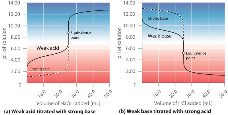
Since this is analogous to the previous section we will only write out the equations that were derived above, but their derivations are similar, it is just that the role of the acid and base switched.
Pure Base
Salt of Weak Base (review section 16.5.5 and 16)
\[\large{pOH=-\log\sqrt{K_{b}[B]_{i}}}\]
(convert to pH if needed)
Buffer Region
Buffer of Weak Base and its Salt (review section 17.2.2.2 and 17.2.4)
\[pOH=pK_b+log\frac{[BH^+]}{B}\]
(convert to pH if needed)
Equivalence point
Salt of Weak Base (review section 16.5.7)
\[[H^+]=\sqrt{\left (\frac{K_w}{K_b} \right )[B]_i} \]
Excess Acid Region
\[\large{[H^+] = \frac{M_A\left (V_A-V_{eq} \right )}{V_A+V_{B,i)}}}\]
Reflections on Titration Curves
Figure \(PageIndex{5}\) shows the titration curves of different weak acids and weak bases of varying concentrations. There are several things we notice from these curves, and two are worth further discussion. The first is that the flat region of the curve is near the midpoint, or at half titer, and this is useful in understanding the pH a buffer can maintain constant. The second the equivalence point, and this can be used to understand how an indicator works, and what indicators are appropriate for what buffers.
Buffer pH
The flat region of the curve is the buffer region because moving along the x-axis (adding an acid or base) has the smallest change along the Y axis (\(\Delta\) pH, and the titration curves for all of the acids and bases in figure 17.3.5 are flattest at half titer. It is clear that the pH at which the above buffers operate varies as the ionization constants vary, and the above diagram demonstrates the logic behind the rules in section 17.2.4.1 for and choosing a buffer, that is, you pick an acid with a K value near the pH (or pOH) and adjust the conjugate pair until it reaches that value.
\[pH=pK_a+\log \dfrac{[A^-]}{[HA]}\] .
Note: the titration curve is flattest at half equivalence. This can be demonstrated by the Henderson Hasselbach Equation.
At any time nHA + nA- = nHA(initial), because you started with pure HA and every time an NaOH reacted with an HA, the number of HA went down by one and A- went up by one.
Thought Experiment
Consider a hypothetical titration with just 100 HF molecules (pKa =3.20) to see why the curve is flattest at half. Note, although the Henderson Hasselbach equation is written in terms of concentration, we can use the number of particles as the volume cancels out in the ratio term
\[\dfrac{[A^-]}{[HA]}=\dfrac{[\frac{n_{A^-}}{V_{T}}]}{[\frac{n_{HA}}{V_{T}}]}=\frac{n_{A^-}}{n_{HA}} \nonumber\]
and the Henderson Hasselbach Equation can be written as:
\[pH=pK_a+\log \frac{n_{A^-}}{n_{HA}}. \nonumber\]
Consider a hypothetical titration with just 100 HF
| nHF | nF- | \(pH=pK_a+\log \frac{n_{A^-}}{n_{HA}}\) | pH |
|---|---|---|---|
| 50 | 50 | \(pH=3.20+\log \frac{50}{50}\) | 3.2 |
| 49 | 51 | \(pH=3.20+\log \frac{51}{49}\) | 3.217 |
| 4 | 96 | \(pH=3.20+\log \frac{96}{4}\) | 4.58 |
| 3 | 97 | \(pH=3.20+\log \frac{97}{3}\) | 4.71 |
Table\(PageIndex{1}\): Hypothetical titration on absurd atom level to give a feel for the ratio term of the buffer equation.
What this shows is that the equation is flattest near half equivalence, which is when it is the best buffer, and so even though there was still an HF to neutralize the 96th NaOH added, the pH went up by 0.13, as compared to 0.017 at half equivalence.
Indicators
Acid base indicators are acids and bases that undergo a color change as they gain or lose a proton, and very dilute solutions of the colored form can be seen by the unaided eye. These are typically organic molecules in nature, and they can be used to estimate the equivalence point if the pH at which they change color is the pH of the equivalence point. Note, when you use an indicator you have an End Point, which is when you stop a titration because the indicator changed color. The Equivalence Point is when the moles acid equals moles base. If the end point of an indicator is at the same pH as the equivalence point, that indicator can be used to determine when the equivalence point is reached.
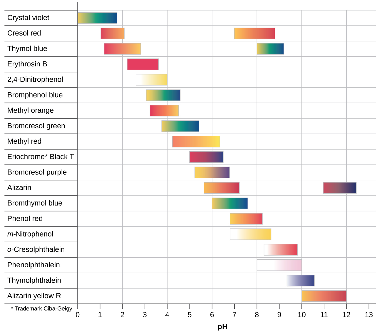
Table\(\PageIndex{2}\): Color changes for some common pH indicators as a function of pH. Note, some diprotic indicators have different colors for the acidic, acid salt, and salt forms.
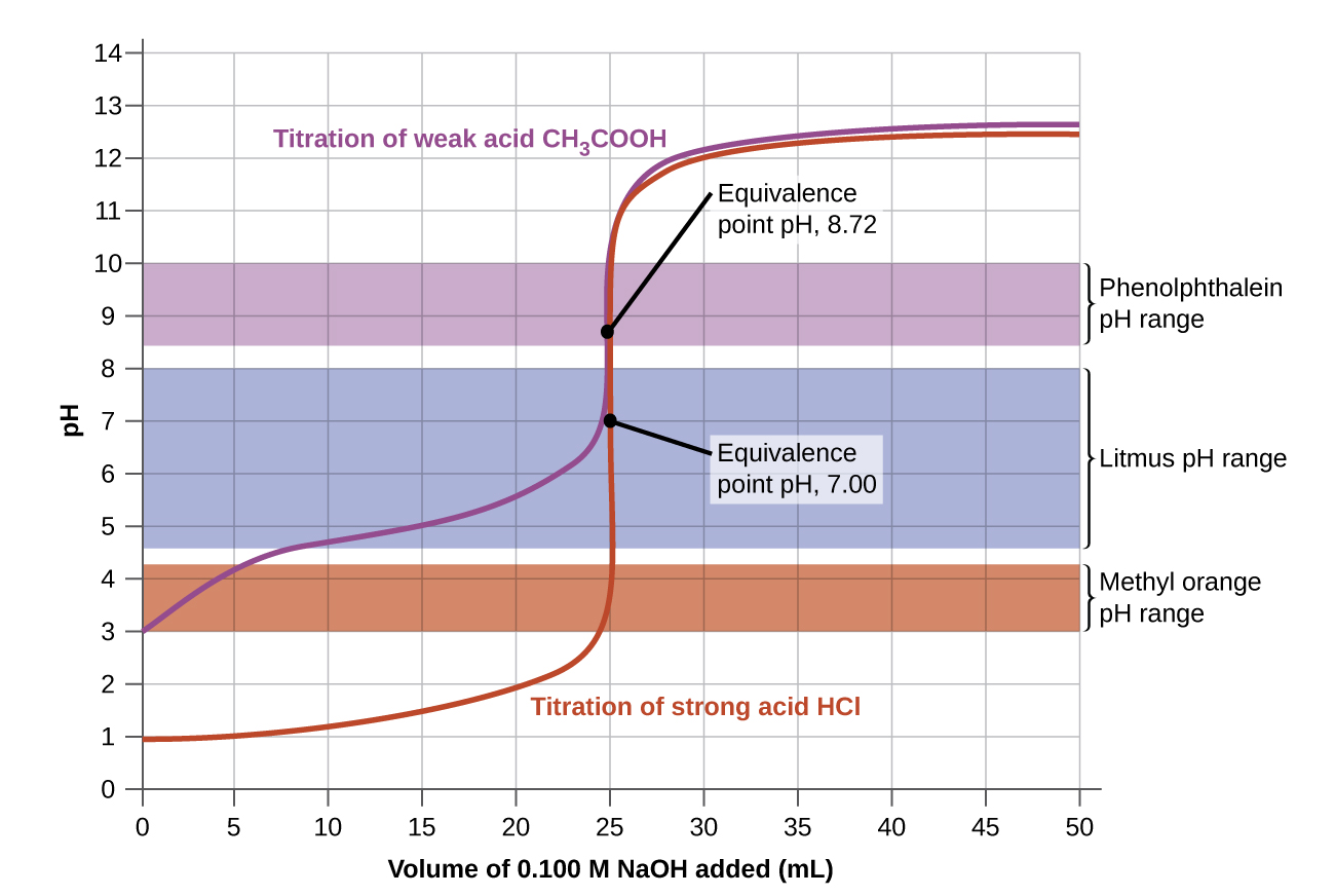
The trick is to identify the pH at the equivalence point (the salt of the compound you are titrating) and pick an indicator that changes pH over that range. A properly picked indicator will change color over a drop, as the line is almost vertical at the equivalence point. An improperly picked indicator will change color very slowly, for example, if you used Bromocresol purple which goes from yellow to purple over the pH range of 5 to 7 (table 17.3.2) and applied it to acetic acid (figure 17.3.6), it would start to change colors around 15 mL and would finish around 25. But an indicator like phenylphthalein would change color at 25 mL.
Polyprotic Titration Curves
Polyprotic acids were covered in sections 16.1.2,16.3.5 and 16.5.8 and it was shown that each proton had its own ionization constant, with \[K_{a1}>K_{a2}>K_{a3}\] . This results in a titration curve like that of figure 17.3.7. If each subsequent Ka is at least a 1000 times smaller than the previous than the protons are taking off stepwise, then there would be a unique equivalence point for each step. In a monoprotic titration and base after the equivalence point is excess and the solution quickly becomes basic. But if there is a leveling off, that could indicate another titratable proton.
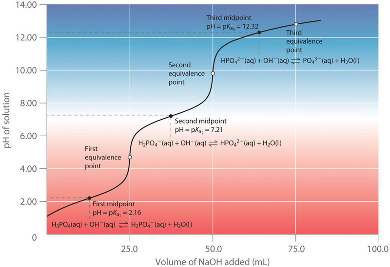
Note, if the Ka values of two successive deprotonations are close to each other, the curve begins to look more like a line and you do not have distinct equivalence points where just one acid salt exists.
Test Yourself
Homework: Section 17.3
Contributors and Attributions
Robert E. Belford (University of Arkansas Little Rock; Department of Chemistry). The breadth, depth and veracity of this work is the responsibility of Robert E. Belford, rebelford@ualr.edu. You should contact him if you have any concerns. This material has both original contributions, and content built upon prior contributions of the LibreTexts Community and other resources, including but not limited to: