4.2: Chemical Reaction Rates

Learning Objectives

• Define chemical reaction rate
• Derive rate expressions from the balanced equation for a given chemical reaction
• Calculate reaction rates from experimental data

A rate is a measure of how some property varies with time. Speed is a familiar rate that expresses the distance traveled by an object in a given amount of time. Wage is a rate that represents the amount of money earned by a person working for a given amount of time. Likewise, the rate of a chemical reaction is a measure of how much reactant is consumed, or how much product is produced, by the reaction in a given amount of time.

The rate of reaction is the change in the amount of a reactant or product per unit time. Reaction rates are therefore determined by measuring the time dependence of some property that can be related to reactant or product amounts. Rates of reactions that consume or produce gaseous substances, for example, are conveniently determined by measuring changes in volume or pressure. For reactions involving one or more colored substances, rates may be monitored via measurements of light absorption. For reactions involving aqueous electrolytes, rates may be measured via changes in a solution’s conductivity.

The progress of a simple reaction (A → B) is shown in (Figure \(\PageIndex{1}\)); the beakers are snapshots of the composition of the solution at 10 s intervals. The number of molecules of reactant (A) and product (B) are plotted as a function of time in the graph. Each point in the graph corresponds to one beaker in (Figure \(\PageIndex{1}\)). The reaction rate is the change in the concentration of either the reactant or the product over a period of time. The concentration of A decreases with time, while the concentration of B increases with time.

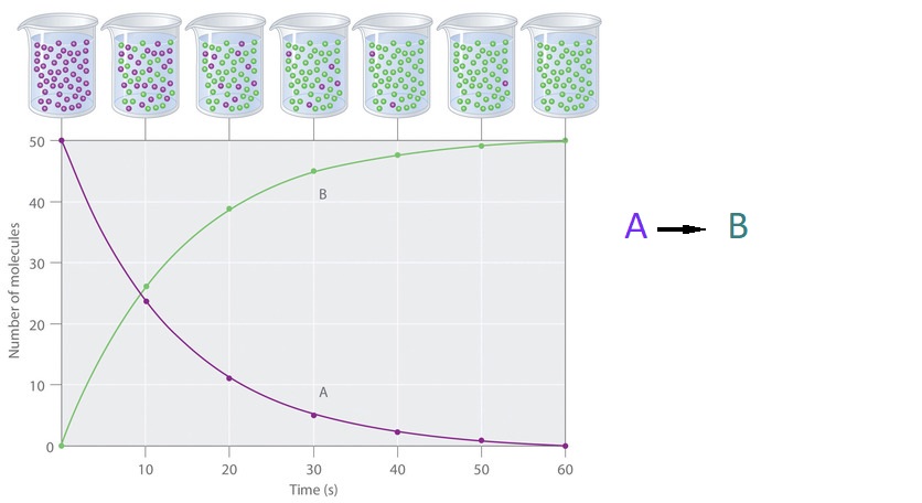
Figure \(\PageIndex{1}\): The Progress of a Simple Reaction (A → B). The mixture initially contains only A molecules (purple). Over time, the number of A molecules decreases and more B molecules (green) are formed (top). The graph shows the change in the number of A and B molecules in the reaction as a function of time over a 1 min period (bottom).

\[\text { rate }=\frac{\Delta[\mathrm{B}]}{\Delta t}=-\frac{\Delta[\mathrm{A}]}{\Delta t}\]

Square brackets indicate molar concentrations, and the capital Greek delta (Δ) means “change in.” Because chemists follow the convention of expressing all reaction rates as positive numbers, however, a negative sign is inserted in front of Δ[A]/Δt to convert that expression to a positive number. The formula shows that the rate of the reaction is equal to the negative of the rate of disappearance of A, and is equal to the rate of appearance of B.

For reactants and products in solution, their relative amounts (concentrations) are conveniently used for purposes of expressing reaction rates. If we measure the concentration of hydrogen peroxide, H₂O₂, in an aqueous solution, we find that it changes slowly over time as the H₂O₂ decomposes, according to the equation:

\[\ce{2H2O2}(aq)⟶\ce{2H2O}(l)+\ce{O2}(g) \nonumber \]

The rate at which the hydrogen peroxide decomposes can be expressed in terms of the rate of change of its concentration, as shown here:

\[\begin{align*}
\ce{rate\: of\: decomposition\: of\: H_2O_2}
&=\mathrm{−\dfrac{change\: in\: concentration\: of\: reactant}{time\: interval}}\\[4pt]
&=−\dfrac{[\ce{H2O2}]_{t_2}−[\ce{H2O2}]_{t_1}}{t_2−t_1}\\[4pt]
&=−\dfrac{Δ[\ce{H2O2}]}{Δt}
\end{align*} \nonumber \]

This mathematical representation of the change in species concentration over time is the rate expression for the reaction. The brackets indicate molar concentrations, and the symbol delta (Δ) indicates “change in.” Thus, \([\ce{H2O2}]_{t_1}\) represents the molar concentration of hydrogen peroxide at some time t₁; likewise, \([\ce{H2O2}]_{t_2}\) represents the molar concentration of hydrogen peroxide at a later time t₂; and Δ[H₂O₂] represents the change in molar concentration of hydrogen peroxide during the time interval Δt (that is, t₂ − t₁). Since the reactant concentration decreases as the reaction proceeds, Δ[H₂O₂] is a negative quantity; we place a negative sign in front of the expression because reaction rates are, by convention, positive quantities. Figure \(\PageIndex{1}\) provides an example of data collected during the decomposition of H₂O₂.

Figure \(\PageIndex{2}\): The rate of decomposition of H₂O₂ in an aqueous solution decreases as the concentration of H₂O₂ decreases.

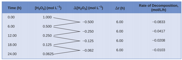
To obtain the tabulated results for this decomposition, the concentration of hydrogen peroxide was measured every 6 hours over the course of a day at a constant temperature of 40 °C. Reaction rates were computed for each time interval by dividing the change in concentration by the corresponding time increment, as shown here for the first 6-hour period:

\[\dfrac{−Δ[\ce{H2O2}]}{Δt}=\mathrm{\dfrac{−(0.500\: mol/L−1.000\: mol/L)}{(6.00\: h−0.00\: h)}=0.0833\: mol\:L^{−1}\:h^{−1}} \nonumber \]

Notice that the reaction rates vary with time, decreasing as the reaction proceeds. Results for the last 6-hour period yield a reaction rate of:

\[\dfrac{−Δ[\ce{H2O2}]}{Δt}=\mathrm{\dfrac{−(0.0625\:mol/L−0.125\:mol/L)}{(24.00\:h−18.00\:h)}=0.0104\:mol\:L^{−1}\:h^{−1}} \nonumber \]

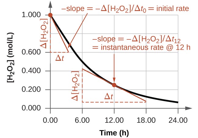
This behavior indicates the reaction continually slows with time. Using the concentrations at the beginning and end of a time period over which the reaction rate is changing results in the calculation of an average rate for the reaction over this time interval. At any specific time, the rate at which a reaction is proceeding is known as its instantaneous rate. The instantaneous rate of a reaction at “time zero,” when the reaction commences, is its initial rate. Consider the analogy of a car slowing down as it approaches a stop sign. The vehicle’s initial rate—analogous to the beginning of a chemical reaction—would be the speedometer reading at the moment the driver begins pressing the brakes (t₀). A few moments later, the instantaneous rate at a specific moment—call it t₁—would be somewhat slower, as indicated by the speedometer reading at that point in time. As time passes, the instantaneous rate will continue to fall until it reaches zero, when the car (or reaction) stops. Unlike instantaneous speed, the car’s average speed is not indicated by the speedometer; but it can be calculated as the ratio of the distance traveled to the time required to bring the vehicle to a complete stop (Δt). Like the decelerating car, the average rate of a chemical reaction will fall somewhere between its initial and final rates.

The instantaneous rate of a reaction may be determined one of two ways. If experimental conditions permit the measurement of concentration changes over very short time intervals, then average rates computed as described earlier provide reasonably good approximations of instantaneous rates. Alternatively, a graphical procedure may be used that, in effect, yields the results that would be obtained if short time interval measurements were possible. If we plot the concentration of hydrogen peroxide against time, the instantaneous rate of decomposition of H₂O₂ at any time t is given by the slope of a straight line that is tangent to the curve at that time (Figure \(\PageIndex{2}\)). We can use calculus to evaluating the slopes of such tangent lines, but the procedure for doing so is beyond the scope of this chapter.

Figure \(\PageIndex{3}\): This graph shows a plot of concentration versus time for a 1.000 M solution of H₂O₂. The rate at any instant is equal to the opposite of the slope of a line tangential to this curve at that time. Tangents are shown at t = 0 h (“initial rate”) and at t = 12 h (“instantaneous rate” at that particular time).

Reaction Rates in Analysis: Test Strips for Urinalysis

Physicians often use disposable test strips to measure the amounts of various substances in a patient’s urine (Figure \(\PageIndex{4}\)). These test strips contain various chemical reagents, embedded in small pads at various locations along the strip, which undergo changes in color upon exposure to sufficient concentrations of specific substances. The usage instructions for test strips often stress that proper read time is critical for optimal results. This emphasis on read time suggests that kinetic aspects of the chemical reactions occurring on the test strip are important considerations.

The test for urinary glucose relies on a two-step process represented by the chemical equations shown here:

\[\ce{C6H12O6 + O2}\underset{\large\textrm{catalyst}}{\xrightarrow{\hspace{45px}}}\ce{C6H10O6 + H2O2} \label{eq1} \]

\[\ce{2H2O2 + 2I-}\underset{\large\textrm{catalyst}}{\xrightarrow{\hspace{45px}}}\ce{I2 + 2H2O + O2} \label{eq2} \]

Equation \(\ref{eq1}\) depicts the oxidation of glucose in the urine to yield glucolactone and hydrogen peroxide. The hydrogen peroxide produced subsequently oxidizes colorless iodide ion to yield brown iodine (Equation \(\ref{eq2}\)), which may be visually detected. Some strips include an additional substance that reacts with iodine to produce a more distinct color change.

The two test reactions shown above are inherently very slow, but their rates are increased by special enzymes embedded in the test strip pad. This is an example of catalysis, a topic discussed later in this chapter. A typical glucose test strip for use with urine requires approximately 30 seconds for completion of the color-forming reactions. Reading the result too soon might lead one to conclude that the glucose concentration of the urine sample is lower than it actually is (a false-negative result). Waiting too long to assess the color change can lead to a false positive due to the slower (not catalyzed) oxidation of iodide ion by other substances found in urine.

Figure \(\PageIndex{4}\): Test strips are commonly used to detect the presence of specific substances in a person’s urine. Many test strips have several pads containing various reagents to permit the detection of multiple substances on a single strip. (credit: Iqbal Osman).

Relative Rates of Reaction

The rate of a reaction may be expressed in terms of the change in the amount of any reactant or product, and may be simply derived from the stoichiometry of the reaction.

For a balanced reaction equation:

\[\ce{aA} + {bB} ⟶\ce{cC} + \ce{dD} \nonumber \]

The rate can be expressed in terms of the decrease in reactant concentration over time or increase in product concentration over time using the stoichiometric coefficients:

\[\text { rate }=-\left(\frac{1}{\mathrm{a}}\right)\left(\frac{\Delta \mathrm{[A]}}{\Delta t}\right)=-\left(\frac{1}{\mathrm{~b}}\right)\left(\frac{\Delta \mathrm{[B]}}{\Delta t}\right) = \left(\frac{1}{\mathrm{~c}}\right)\left(\frac{\Delta \mathrm{[C]}}{\Delta t}\right) = \left(\frac{1}{\mathrm{~d}}\right)\left(\frac{\Delta \mathrm{[D]}}{\Delta t}\right)\]

Reaction rate is positive, so rate of reaction is equal to the negative of the rate of disappearance of reactants.

Consider the reaction represented by the following equation:

\[\ce{2NH3}(g)⟶\ce{N2}(g)+\ce{3H2}(g) \nonumber \]

The stoichiometric factors derived from this equation may be used to relate reaction rates in the same manner that they are used to related reactant and product amounts. The relation between the reaction rates expressed in terms of nitrogen production and ammonia consumption, for example, is:

\[\mathrm{−\dfrac{Δmol\: NH_3}{Δ\mathit t}×\dfrac{1\: mol\: N_2}{2\: mol\: NH_3}=\dfrac{Δmol\:N_2}{Δ\mathit t}} \nonumber \]

We can express this more simply without showing the stoichiometric factor’s units:

\[−\dfrac{1}{2}\dfrac{\mathrm{Δmol\:NH_3}}{Δt}=\dfrac{\mathrm{Δmol\:N_2}}{Δt} \nonumber \]

Note that a negative sign has been added to account for the opposite signs of the two amount changes (the reactant amount is decreasing while the product amount is increasing). If the reactants and products are present in the same solution, the molar amounts may be replaced by concentrations:

\[−\dfrac{1}{2}\dfrac{Δ[\ce{NH3}]}{Δt}=\dfrac{Δ[\ce{N2}]}{Δt} \nonumber \]

Similarly, the rate of formation of H₂ is three times the rate of formation of N₂ because three moles of H₂ form during the time required for the formation of one mole of N₂:

\[\dfrac{1}{3}\dfrac{Δ[\ce{H2}]}{Δt}=\dfrac{Δ[\ce{N2}]}{Δt} \nonumber \]

Figure \(\PageIndex{3}\) illustrates the change in concentrations over time for the decomposition of ammonia into nitrogen and hydrogen at 1100 °C. We can see from the slopes of the tangents drawn at t = 500 seconds that the instantaneous rates of change in the concentrations of the reactants and products are related by their stoichiometric factors. The rate of hydrogen production, for example, is observed to be three times greater than that for nitrogen production:

\[\dfrac{2.91×10^{−6}\:M/\ce s}{9.71×10^{−6}\:M/\ce s}≈3 \nonumber \]

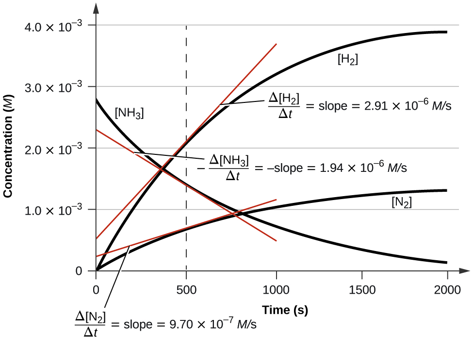
Figure \(\PageIndex{3}\): This graph shows the changes in concentrations of the reactants and products during the reaction \(\ce{2NH3⟶N2 + 3H2}\). The rates of change of the three concentrations are related by their stoichiometric factors, as shown by the different slopes of the tangents at t = 500 s.

Example \(\PageIndex{1}\)

Consider the conversion of dinitrogen tetroxide, N₂O₄ (g) to nitrogen dioxide, NO₂ (g):

\[ \mathrm{N}_2 \mathrm{O}_4(\mathrm{~g}) \ ⟶ 2 \mathrm{NO}_2(\mathrm{~g}) \nonumber\]

Write the rate expression for the reaction in terms of disappearance of the reactants and appearance of the products.

Solution

For every one mole of reactant that disappears, two moles of product are formed. The rate of disappearance of N₂O₄ must be must be half of the rate of appearance of NO₂. The rate of reaction therefore may be expressed as:

\[\text { rate } = −\dfrac{\mathrm{Δ[\:N_2O_4]}}{Δt}=\dfrac{1}{2}\dfrac{\mathrm{Δ[\:NO_2]}}{Δt} \nonumber \]

Example \(\PageIndex{2}\): Expressions for Relative Reaction Rates

The first step in the production of nitric acid is the combustion of ammonia:

\[\ce{4NH3}(g)+\ce{5O2}(g)⟶\ce{4NO}(g)+\ce{6H2O}(g) \nonumber \]

Write the equations that relate the rates of consumption of the reactants and the rates of formation of the products.

Solution

Considering the stoichiometry of this homogeneous reaction, the rates for the consumption of reactants and formation of products are:

\[−\dfrac{1}{4}\dfrac{Δ[\ce{NH3}]}{Δt}=−\dfrac{1}{5}\dfrac{Δ[\ce{O2}]}{Δt}=\dfrac{1}{4}\dfrac{Δ[\ce{NO}]}{Δt}=\dfrac{1}{6}\dfrac{Δ[\ce{H2O}]}{Δt} \nonumber \]

Exercise \(\PageIndex{1}\)

The rate of formation of Br₂ is 6.0 × 10⁻⁶ mol/L/s in a reaction described by the following net ionic equation:

\[\ce{5Br- + BrO3- + 6H+ ⟶ 3Br2 + 3H2O} \nonumber \]

Write the equations that relate the rates of consumption of the reactants and the rates of formation of the products.

Answer

\[−\dfrac{1}{5}\dfrac{Δ[\ce{Br-}]}{Δt}=−\dfrac{Δ[\ce{BrO3-}]}{Δt}=−\dfrac{1}{6}\dfrac{Δ[\ce{H+}]}{Δt}=\dfrac{1}{3}\dfrac{Δ[\ce{Br2}]}{Δt}=\dfrac{1}{3}\dfrac{Δ[\ce{H2O}]}{Δt} \nonumber \]

Example \(\PageIndex{3}\): Reaction Rate Expressions for Decomposition of H₂O₂

The graph in Figure \(\PageIndex{3}\) shows the rate of the decomposition of H₂O₂ over time:

\[\ce{2H2O2 ⟶ 2H2O + O2} \nonumber \]

Based on these data, the instantaneous rate of decomposition of H₂O₂ at t = 11.1 h is determined to be 3.20 × 10⁻² mol/L/h, that is:

\[−\dfrac{Δ[\ce{H2O2}]}{Δt}=\mathrm{3.20×10^{−2}\:mol\: L^{−1}\:h^{−1}} \nonumber \]

What is the instantaneous rate of production of H₂O and O₂?

Solution

Using the stoichiometry of the reaction, we may determine that:

\[−\dfrac{1}{2}\dfrac{Δ[\ce{H2O2}]}{Δt}=\dfrac{1}{2}\dfrac{Δ[\ce{H2O}]}{Δt}=\dfrac{Δ[\ce{O2}]}{Δt} \nonumber \]

Therefore:

\[\mathrm{\dfrac{1}{2}×3.20×10^{−2}\:mol\:L^{−1}\:h^{−1}}=\dfrac{Δ[\ce{O2}]}{Δt} \nonumber \]

and

\[\dfrac{Δ[\ce{O2}]}{Δt}=\mathrm{1.60×10^{−2}\:mol\:L^{−1}\:h^{−1}} \nonumber \]

Exercise \(\PageIndex{2}\)

If the rate of decomposition of ammonia, NH₃, at 1150 K is 2.10 × 10⁻⁶ mol/L/s, what is the rate of production of nitrogen and hydrogen?

Answer

1.05 × 10⁻⁶ mol/L/s, N₂ and 3.15 × 10⁻⁶ mol/L/s, H₂.

Summary

The rate of a reaction can be expressed either in terms of the decrease in the amount of a reactant or the increase in the amount of a product per unit time. Relations between different rate expressions for a given reaction are derived directly from the stoichiometric coefficients of the equation representing the reaction.

Glossary

average rate

rate of a chemical reaction computed as the ratio of a measured change in amount or concentration of substance to the time interval over which the change occurred

initial rate

instantaneous rate of a chemical reaction at t = 0 s (immediately after the reaction has begun)

instantaneous rate

rate of a chemical reaction at any instant in time, determined by the slope of the line tangential to a graph of concentration as a function of time

rate of reaction

measure of the speed at which a chemical reaction takes place

rate expression

mathematical representation relating reaction rate to changes in amount, concentration, or pressure of reactant or product species per unit time