3.2: Periodic Variations in Element Properties

Learning Objectives

• Describe and explain the observed trends in atomic size, ionization energy, and electron affinity of the elements

The elements in groups (vertical columns) of the periodic table exhibit similar chemical behavior. This similarity occurs because the members of a group have the same number and distribution of electrons in their valence shells. However, there are also other patterns in chemical properties on the periodic table. For example, as we move down a group, the metallic character of the atoms increases. Oxygen, at the top of Group 16 (6A), is a colorless gas; in the middle of the group, selenium is a semiconducting solid; and, toward the bottom, polonium is a silver-grey solid that conducts electricity.

As we go across a period from left to right, we add a proton to the nucleus and an electron to the valence shell with each successive element. As we go down the elements in a group, the number of electrons in the valence shell remains constant, but the principal quantum number increases by one each time. An understanding of the electronic structure of the elements allows us to examine some of the properties that govern their chemical behavior. These properties vary periodically as the electronic structure of the elements changes. They are (1) size (radius) of atoms and ions, (2) ionization energies, and (3) electron affinities.

Effective Nuclear Charge: Penetration and Shielding

Electrons are negatively charged and are pulled pretty close to each other by their attraction to the positive charge of a nucleus. The electrons are attracted to the nucleus at the same time as electrons repel each other. The balance between attractive and repulsive forces results in shielding. The orbital (n) and subshell (m_l) define how close an electron can approach the nucleus. The ability of an electron to get close to the nucleus is penetration.

The force that an electron feels is dependent on the distance from the nearest charge (i.e., an electron, usually with bigger atoms and on the outer shells) and the amount of charge. More distance between the charges will result in less force, and more charge will have more force of attraction or repulsion.

In the simplest case, every electron in an atom would feel the same amount of "pull" from the nucleus. For example, in Li, all three electrons might "feel" the +3 charge from the nucleus. However, this is not the case when observing atomic behavior. When considering the core electrons (or the electrons closest to the nucleus), the nuclear charge "felt" by the electrons (Effective Nuclear Charge (Zeff) is close to the actual nuclear charge. As you proceed from the core electrons to the outer valence electrons, Zeff falls significantly. This is because of shielding, or simply the electrons closest to the nucleus decrease the amount of nuclear charge affecting the outer electrons. Shielding is caused by the combination of partial neutralization of nuclear charge by core electrons, and by electron-electron repulsion.

The amount of charge felt by an electron depends on its distance from the nucleus. The closer an electron comes to the nucleus, or the more it penetrates, the stronger its attraction to the nucleus. Core electrons penetrate more and feel more of the nucleus than the other electrons.

Orbital Penetration

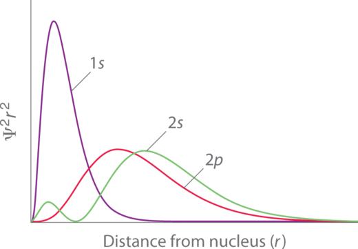
Penetration describes the proximity to which an electron can approach to the nucleus. In a multi-electron system, electron penetration is defined by an electron's relative electron density (probability density) near the nucleus of an atom. Electrons in different orbitals have different wavefunctions and therefore different radial distributions and probabilities (defined by quantum numbers n and m_l around the nucleus). In other words, penetration depends on the shell (n) and subshell (m_l). For example, we see that since a 2s electron has more electron density near the nucleus than a 2p electron, it is penetrating the nucleus of the atom more than the 2p electron. The penetration power of an electron, in a multi-electron atom, is dependent on the values of both the shell and subshell.

Within the same shell value (n), the penetrating power of an electron follows this trend in subshells (m_l):

s>p>d>f

And for different values of shell (n) and subshell (l), penetrating power of an electron follows this trend:

1s>2s>2p>3s>3p>4s>3d>4p>5s>4d>5p>6s>4f....

and the energy of an electron for each shell and subshell goes as follows...

1s<2s<2p<3s<3p<4s<3d<4p....

The electron probability density for s-orbitals is highest in the center of the orbital, or at the nucleus. If we imagine a dartboard that represents the circular shape of the s-orbital and if the darts landed in correlation to the probability to where and electron would be found, the greatest dart density would be at the 50 points region but most of the darts would be at the 30 point region. When considering the 1s-orbital, the spherical shell of 53 pm is represented by the 30 point ring.

Electrons which experience greater penetration experience stronger attraction to the nucleus, less shielding, and therefore experience a larger Effective Nuclear Charge (Zeff), but shield other electrons more effectively.

Shielding

An atom (assuming its atomic number is greater than 2) has core electrons that are extremely attracted to the nucleus in the middle of the atom. However the number of protons in the nucleus are never equal to the number of core electrons (relatively) adjacent to the nucleus. The number of protons increase by one across the periodic table, but the number of core electrons change by periods. The first period has no core electrons, the second has 2, the third has 10, and etc. This number is not equal to the number of protons. So that means that the core electrons feel a stronger pull towards the nucleus than any other electron within the system. The valence electrons are farther out from the nucleus, so they experience a smaller force of attraction.

Shielding refers to the core electrons repelling the outer rings and thus lowering the 1:1 ratio. Hence, the nucleus has "less grip" on the outer electrons and are shielded from them. Electrons that have greater penetration can get closer to the nucleus and effectively block out the charge from electrons that have less proximity. For example, Zeff is calculated by subtracting the magnitude of shielding from the total nuclear charge. The value of Zeff will provide information on how much of a charge an electron actually experiences.

\(\PageIndex{1}\): This image shows how inner electrons can shield outer electrons from the nuclear charge. (CC BY-SA 3.0; from Wikipedia).

Because the order of electron penetration from greatest to least is s, p, d, f; the order of the amount of shielding done is also in the order s, p, d, f.

Since the 2s electron has more density near the nucleus of an atom than a 2p electron, it is said to shield the 2p electron from the full effective charge of the nucleus. Therefore the 2p electron feels a lesser effect of the positively charged nucleus of the atom due to the shielding ability of the electrons closer to the nucleus than itself, (i.e. 2s electron).

These electrons that are shielded from the full charge of the nucleus are said to experience an effective nuclear charge (Zeff) of the nucleus, which is some degree less than the full nuclear charge an electron would feel in a hydrogen atom or hydrogenlike ions. The effective nuclear charge of an atom is given by the equation:

Zeff=Z−S

where

• Z is the atomic number (number of protons in nucleus) and
• S is the shielding constant

We can see from this equation that the effective nuclear charge of an atom increases as the number of protons in an atom increases. Therefore as we go from left to right on the periodic table the effective nuclear charge of an atom increases in strength and holds the outer electrons closer and tighter to the nucleus. This phenomena can explain the decrease in atomic radii we see as we go across the periodic table as electrons are held closer to the nucleus due to increase in number of protons and increase in effective nuclear charge.

Example 1: Fluorine, Neon, and Sodium

What is the effective attraction Zeff experienced by the valence electrons in the three isoelectronic species: the fluorine anion, the neutral neon atom, and sodium cation?

Solution

Each species has 10 electrons, and the number of nonvalence electrons is 2 (10 total electrons - 8 valence) but the effective nuclear charge varies because each has a different atomic number A.

The charge Z of the nucleus of a fluorine atom is 9, but the valence electrons are screened appreciably by the core electrons (four electrons from the 1s and 2s orbitals) and partially by the 7 electrons in the 2p orbitals.

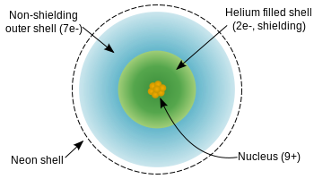
Diagram of a fluorine atom showing the extent of effective nuclear charge. (CC BY-SA- 3.0; Wikipedia).

• Zeff(F−)=9−2=7+
• Zeff(Ne)=10−2=8+
• Zeff(Na+)=11−2=9+

So the sodium cation has the greatest effective nuclear charge, and thus the smallest radius.

Radial Distribution Graphs

A radial distribution function graph describes the distribution of orbitals with the effects of shielding (Figure \(\PageIndex{2}\) ). The small peak of the 2s orbital shows that he electrons in the 2s orbital are closest to the nucleus. Therefore, it is the electrons in the 2p orbital of Be that are being shielded from the nucleus, by the electrons in the 2s orbital. The following is the radial distribution of the 1s and 2s orbitals. Notice the 1s orbital is shifted to the right, while the 2s orbital has a node.

Figure \(\PageIndex{2}\) : Orbital Penetration. A comparison of the radial probability distribution of the 2s and 2p orbitals for various states of the hydrogen atom shows that the 2s orbital penetrates inside the 1s orbital more than the 2p orbital does. Consequently, when an electron is in the small inner lobe of the 2s orbital, it experiences a relatively large value of Zeff, which causes the energy of the 2s orbital to be lower than the energy of the 2p orbital.

Periodic Trends Due to Penetration and Shielding

• Effective Nuclear Charge (ZeffZeff): The effective nuclear charge increases from left to right and increases from top to bottom on the periodic table.
• Atomic Radius: The atomic radius decreases from left to right, and increases from top to bottom.
• Ionization Energies: The ionization energies increase from left to right, and decrease from top to bottom.
• Electronegativity: The electronegativity of the elements is highest near flourine. In general, it increases from left to right and decreases from top to bottom.

Variation in Covalent Radius

The quantum mechanical picture makes it difficult to establish a definite size of an atom. However, there are several practical ways to define the radius of atoms and, thus, to determine their relative sizes that give roughly similar values. We will use the covalent radius (Figure \(\PageIndex{3}\)), which is defined as one-half the distance between the nuclei of two identical atoms when they are joined by a covalent bond (this measurement is possible because atoms within molecules still retain much of their atomic identity).

Figure \(\PageIndex{3}\): (a) The radius of an atom is defined as one-half the distance between the nuclei in a molecule consisting of two identical atoms joined by a covalent bond. The atomic radius for the halogens increases down the group as n increases. (b) Covalent radii of the elements. The general trend is that radii increase down a group and decrease across a period.

We know that as we scan down a group, the principal quantum number, n, increases by one for each element. Thus, the electrons are being added to a region of space that is increasingly distant from the nucleus. Consequently, the size of the atom (and its covalent radius) must increase as we increase the distance of the outermost electrons from the nucleus. This trend is illustrated for the covalent radii of the halogens in Table \(\PageIndex{1}\) and Figure \(\PageIndex{3}\). The trends for the entire periodic table can be seen in Figure \(\PageIndex{4}\).

Table \(\PageIndex{1}\): Covalent Radii of the Halogen Group Elements

Atom	Covalent radius (pm)	Nuclear charge
F	64	+9
Cl	99	+17
Br	114	+35
I	133	+53
At	148	+85

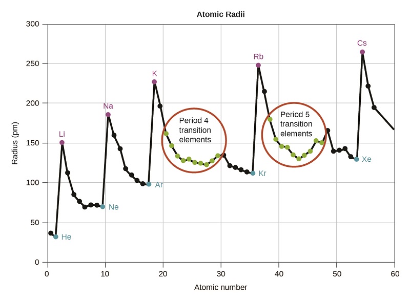
As shown in Figure \(\PageIndex{4}\), as we move across a period from left to right, we generally find that each element has a smaller covalent radius than the element preceding it. This might seem counterintuitive because it implies that atoms with more electrons have a smaller atomic radius. This can be explained with the concept of effective nuclear charge, \(Z_{eff}\). This is the pull exerted on a specific electron by the nucleus, taking into account any electron–electron repulsions. For hydrogen, there is only one electron and so the nuclear charge (Z) and the effective nuclear charge (Z_eff) are equal. For all other atoms, the inner electrons partially shield the outer electrons from the pull of the nucleus, and thus:

\[Z_\ce{eff}=Z−shielding \nonumber \]

Shielding is determined by the probability of another electron being between the electron of interest and the nucleus, as well as by the electron–electron repulsions the electron of interest encounters. Core electrons are adept at shielding, while electrons in the same valence shell do not block the nuclear attraction experienced by each other as efficiently. Thus, each time we move from one element to the next across a period, Z increases by one, but the shielding increases only slightly. Thus, Z_eff increases as we move from left to right across a period. The stronger pull (higher effective nuclear charge) experienced by electrons on the right side of the periodic table draws them closer to the nucleus, making the covalent radii smaller.

Figure \(\PageIndex{4}\): Within each period, the trend in atomic radius decreases as Z increases; for example, from K to Kr. Within each group (e.g., the alkali metals shown in purple), the trend is that atomic radius increases as Z increases.

Thus, as we would expect, the outermost or valence electrons are easiest to remove because they have the highest energies, are shielded more, and are farthest from the nucleus. As a general rule, when the representative elements form cations, they do so by the loss of the ns or np electrons that were added last in the Aufbau process. The transition elements, on the other hand, lose the ns electrons before they begin to lose the (n – 1)d electrons, even though the ns electrons are added first, according to the Aufbau principle.

Example \(\PageIndex{1}\): Sorting Atomic Radii

Predict the order of increasing covalent radius for Ge, Fl, Br, Kr.

Solution

Radius increases as we move down a group, so Ge < Fl (Note: Fl is the symbol for flerovium, element 114, NOT fluorine). Radius decreases as we move across a period, so Kr < Br < Ge. Putting the trends together, we obtain Kr < Br < Ge < Fl.

Exercise \(\PageIndex{1}\)

Give an example of an atom whose size is smaller than fluorine.

Answer

Ne or He

Variation in Ionic Radii

Ionic radius is the measure used to describe the size of an ion. A cation always has fewer electrons and the same number of protons as the parent atom; it is smaller than the atom from which it is derived (Figure \(\PageIndex{5}\)). For example, the covalent radius of an aluminum atom (1s²2s²2p⁶3s²3p¹) is 118 pm, whereas the ionic radius of an Al³⁺ (1s²2s²2p⁶) is 68 pm. As electrons are removed from the outer valence shell, the remaining core electrons occupying smaller shells experience a greater effective nuclear charge Z_eff (as discussed) and are drawn even closer to the nucleus.

Figure \(\PageIndex{5}\): The radius for a cation is smaller than the parent atom (Al), due to the lost electrons; the radius for an anion is larger than the parent (S), due to the gained electrons.

Cations with larger charges are smaller than cations with smaller charges (e.g., V²⁺ has an ionic radius of 79 pm, while that of V³⁺ is 64 pm). Proceeding down the groups of the periodic table, we find that cations of successive elements with the same charge generally have larger radii, corresponding to an increase in the principal quantum number, n.

An anion (negative ion) is formed by the addition of one or more electrons to the valence shell of an atom. This results in a greater repulsion among the electrons and a decrease in \(Z_{eff}\) per electron. Both effects (the increased number of electrons and the decreased Z_eff) cause the radius of an anion to be larger than that of the parent atom ( Figure \(\PageIndex{3}\)). For example, a sulfur atom ([Ne]3s²3p⁴) has a covalent radius of 104 pm, whereas the ionic radius of the sulfide anion ([Ne]3s²3p⁶) is 170 pm. For consecutive elements proceeding down any group, anions have larger principal quantum numbers and, thus, larger radii.

Atoms and ions that have the same electron configuration are said to be isoelectronic. Examples of isoelectronic species are N^3–, O^2–, F^–, Ne, Na⁺, Mg²⁺, and Al³⁺ (1s²2s²2p⁶). Another isoelectronic series is P^3–, S^2–, Cl^–, Ar, K⁺, Ca²⁺, and Sc³⁺ ([Ne]3s²3p⁶). For atoms or ions that are isoelectronic, the number of protons determines the size. The greater the nuclear charge, the smaller the radius in a series of isoelectronic ions and atoms.

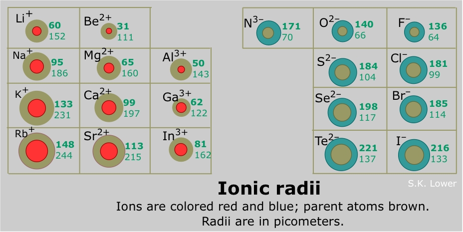Figure \(\PageIndex{6}\): All non-metals (except for the noble gases which do not form ions) form anions which become larger down a group. For non-metals, a subtle trend of decreasing ionic radii is found across a pegroup theoryriod (Shannon 1976). Anions are almost always larger than cations, although there are some exceptions (i.e. fluorides of some alkali metals).

Variation in Ionization Energies

The amount of energy required to remove the most loosely bound electron from a gaseous atom in its ground state is called its first ionization energy (IE₁). The first ionization energy for an element, X, is the energy required to form a cation with +1 charge:

\[\ce{X}(g)⟶\ce{X+}(g)+\ce{e-}\hspace{20px}\ce{IE_1} \nonumber \]

The energy required to remove the second most loosely bound electron is called the second ionization energy (IE₂).

\[\ce{X+}(g)⟶\ce{X^2+}(g)+\ce{e-}\hspace{20px}\ce{IE_2} \nonumber \]

The energy required to remove the third electron is the third ionization energy, and so on. Energy is always required to remove electrons from atoms or ions, so ionization processes are endothermic and IE values are always positive. For larger atoms, the most loosely bound electron is located farther from the nucleus and so is easier to remove. Thus, as size (atomic radius) increases, the ionization energy should decrease. Relating this logic to what we have just learned about radii, we would expect first ionization energies to decrease down a group and to increase across a period.

Figure \(\PageIndex{7}\): The first ionization energy of the elements in the first five periods are plotted against their atomic number.

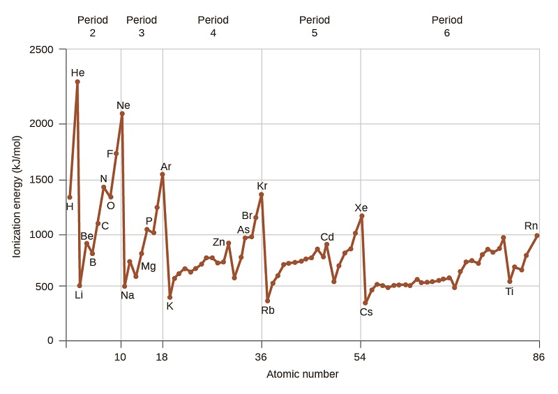
Figure \(\PageIndex{7}\) graphs the relationship between the first ionization energy and the atomic number of several elements. Within a period, the values of first ionization energy for the elements (IE₁) generally increases with increasing Z. Down a group, the IE₁ value generally decreases with increasing Z. There are some systematic deviations from this trend, however. Note that the ionization energy of boron (atomic number 5) is less than that of beryllium (atomic number 4) even though the nuclear charge of boron is greater by one proton. This can be explained because the energy of the subshells increases as l increases, due to penetration and shielding (as discussed previously in this chapter). Within any one shell, the s electrons are lower in energy than the p electrons. This means that an s electron is harder to remove from an atom than a p electron in the same shell. The electron removed during the ionization of beryllium ([He]2s²) is an s electron, whereas the electron removed during the ionization of boron ([He]2s²2p¹) is a p electron; this results in a lower first ionization energy for boron, even though its nuclear charge is greater by one proton. Thus, we see a small deviation from the predicted trend occurring each time a new subshell begins.

Figure \(\PageIndex{8}\): This version of the periodic table shows the first ionization energy of (IE: ₁), in kJ/mol, of selected elements.

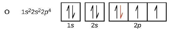
Another deviation occurs as orbitals become more than one-half filled. The first ionization energy for oxygen is slightly less than that for nitrogen, despite the trend in increasing IE₁ values across a period. Looking at the orbital diagram of oxygen, we can see that removing one electron will eliminate the electron–electron repulsion caused by pairing the electrons in the 2p orbital and will result in a half-filled orbital (which is energetically favorable). Analogous changes occur in succeeding periods (note the dip for sulfur after phosphorus in Figure \(\PageIndex{7}\).

Removing an electron from a cation is more difficult than removing an electron from a neutral atom because of the greater electrostatic attraction to the cation. Likewise, removing an electron from a cation with a higher positive charge is more difficult than removing an electron from an ion with a lower charge. Thus, successive ionization energies for one element always increase. As seen in Table \(\PageIndex{2}\), there is a large increase in the ionization energies (color change) for each element. This jump corresponds to removal of the core electrons, which are harder to remove than the valence electrons. For example, Sc and Ga both have three valence electrons, so the rapid increase in ionization energy occurs after the third ionization.

Table \(\PageIndex{2}\): Successive Ionization Energies for Selected Elements (kJ/mol)

Element	IE1	IE2	IE3	IE4	IE5	IE6	IE7
K	418.8	3051.8	4419.6	5876.9	7975.5	9590.6	11343
Ca	589.8	1145.4	4912.4	6490.6	8153.0	10495.7	12272.9
Sc	633.1	1235.0	2388.7	7090.6	8842.9	10679.0	13315.0
Ga	578.8	1979.4	2964.6	6180	8298.7	10873.9	13594.8
Ge	762.2	1537.5	3302.1	4410.6	9021.4	Not available	Not available
As	944.5	1793.6	2735.5	4836.8	6042.9	12311.5	Not available

Example \(\PageIndex{2}\): Ranking Ionization Energies

Predict the order of increasing energy for the following processes: IE₁ for Al, IE₁ for Tl, IE₂ for Na, IE₃ for Al.

Solution

Removing the 6p¹ electron from Tl is easier than removing the 3p¹ electron from Al because the higher n orbital is farther from the nucleus, so IE₁(Tl) < IE₁(Al). Ionizing the third electron from

\[\ce{Al}\hspace{20px}\ce{(Al^2+⟶Al^3+ + e- )} \nonumber \]

requires more energy because the cation Al²⁺ exerts a stronger pull on the electron than the neutral Al atom, so IE₁(Al) < IE₃(Al). The second ionization energy for sodium removes a core electron, which is a much higher energy process than removing valence electrons. Putting this all together, we obtain:

IE₁(Tl) < IE₁(Al) < IE₃(Al) < IE₂(Na).

Exercise \(\PageIndex{2}\)

Which has the lowest value for IE₁: O, Po, Pb, or Ba?

Answer

Ba

Variation in Electron Affinities

The electron affinity [EA] is the energy change for the process of adding an electron to a gaseous atom to form an anion (negative ion).

\[\ce{X}(g)+\ce{e-}⟶\ce{X-}(g)\hspace{20px}\ce{EA_1} \nonumber \]

This process can be either endothermic or exothermic, depending on the element. The EA of some of the elements is given in Figure \(\PageIndex{9}\). You can see that many of these elements have negative values of EA, which means that energy is released when the gaseous atom accepts an electron. However, for some elements, energy is required for the atom to become negatively charged and the value of their EA is positive. Just as with ionization energy, subsequent EA values are associated with forming ions with more charge. The second EA is the energy associated with adding an electron to an anion to form a –2 ion, and so on.

Figure \(\PageIndex{9}\): This version of the periodic table displays the electron affinity values (in kJ/mol) for selected elements.:

As we might predict, it becomes easier to add an electron across a series of atoms as the effective nuclear charge of the atoms increases. We find, as we go from left to right across a period, EAs tend to become more negative. The exceptions found among the elements of group 2 (2A), group 15 (5A), and group 18 (8A) can be understood based on the electronic structure of these groups. The noble gases, group 18 (8A), have a completely filled shell and the incoming electron must be added to a higher n level, which is more difficult to do. Group 2 (2A) has a filled ns subshell, and so the next electron added goes into the higher energy np, so, again, the observed EA value is not as the trend would predict. Finally, group 15 (5A) has a half-filled np subshell and the next electron must be paired with an existing np electron. In all of these cases, the initial relative stability of the electron configuration disrupts the trend in EA.

We also might expect the atom at the top of each group to have the largest EA; their first ionization potentials suggest that these atoms have the largest effective nuclear charges. However, as we move down a group, we see that the second element in the group most often has the greatest EA. The reduction of the EA of the first member can be attributed to the small size of the n = 2 shell and the resulting large electron–electron repulsions. For example, chlorine, with an EA value of –348 kJ/mol, has the highest value of any element in the periodic table. The EA of fluorine is –322 kJ/mol. When we add an electron to a fluorine atom to form a fluoride anion (F^–), we add an electron to the n = 2 shell. The electron is attracted to the nucleus, but there is also significant repulsion from the other electrons already present in this small valence shell. The chlorine atom has the same electron configuration in the valence shell, but because the entering electron is going into the n = 3 shell, it occupies a considerably larger region of space and the electron–electron repulsions are reduced. The entering electron does not experience as much repulsion and the chlorine atom accepts an additional electron more readily.

The properties discussed in this section (size of atoms and ions, effective nuclear charge, ionization energies, and electron affinities) are central to understanding chemical reactivity. For example, because fluorine has an energetically favorable EA and a large energy barrier to ionization (IE), it is much easier to form fluorine anions than cations. Metallic properties including conductivity and malleability (the ability to be formed into sheets) depend on having electrons that can be removed easily. Thus, metallic character increases as we move down a group and decreases across a period in the same trend observed for atomic size because it is easier to remove an electron that is farther away from the nucleus.

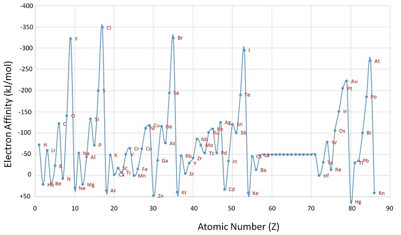
Figure \(\PageIndex{10}\): A Plot of Periodic Variation of Electron Affinity with Atomic Number for the First Six Rows of the Periodic Table. Notice that electron affinities can be both negative and positive. from Robert J. Lancashire (University of the West Indies).

Summary

Electron configurations allow us to understand many periodic trends. Covalent radius increases as we move down a group because the n level (orbital size) increases. Covalent radius mostly decreases as we move left to right across a period because the effective nuclear charge experienced by the electrons increases, and the electrons are pulled in tighter to the nucleus. Anionic radii are larger than the parent atom, while cationic radii are smaller, because the number of valence electrons has changed while the nuclear charge has remained constant. Ionization energy (the energy associated with forming a cation) decreases down a group and mostly increases across a period because it is easier to remove an electron from a larger, higher energy orbital. Electron affinity (the energy associated with forming an anion) is more favorable (exothermic) when electrons are placed into lower energy orbitals, closer to the nucleus. Therefore, electron affinity becomes increasingly negative as we move left to right across the periodic table and decreases as we move down a group. For both IE and electron affinity data, there are exceptions to the trends when dealing with completely filled or half-filled subshells.

Glossary

covalent radius

one-half the distance between the nuclei of two identical atoms when they are joined by a covalent bond

effective nuclear charge

charge that leads to the Coulomb force exerted by the nucleus on an electron, calculated as the nuclear charge minus shielding

electron affinity

energy required to add an electron to a gaseous atom to form an anion

ionization energy

energy required to remove an electron from a gaseous atom or ion. The associated number (e.g., second ionization energy) corresponds to the charge of the ion produced (X²⁺)

isoelectronic

group of ions or atoms that have identical electron configurations