J-Coupling (Scalar)
- Page ID
- 1826
\( \newcommand{\vecs}[1]{\overset { \scriptstyle \rightharpoonup} {\mathbf{#1}} } \)
\( \newcommand{\vecd}[1]{\overset{-\!-\!\rightharpoonup}{\vphantom{a}\smash {#1}}} \)
\( \newcommand{\dsum}{\displaystyle\sum\limits} \)
\( \newcommand{\dint}{\displaystyle\int\limits} \)
\( \newcommand{\dlim}{\displaystyle\lim\limits} \)
\( \newcommand{\id}{\mathrm{id}}\) \( \newcommand{\Span}{\mathrm{span}}\)
( \newcommand{\kernel}{\mathrm{null}\,}\) \( \newcommand{\range}{\mathrm{range}\,}\)
\( \newcommand{\RealPart}{\mathrm{Re}}\) \( \newcommand{\ImaginaryPart}{\mathrm{Im}}\)
\( \newcommand{\Argument}{\mathrm{Arg}}\) \( \newcommand{\norm}[1]{\| #1 \|}\)
\( \newcommand{\inner}[2]{\langle #1, #2 \rangle}\)
\( \newcommand{\Span}{\mathrm{span}}\)
\( \newcommand{\id}{\mathrm{id}}\)
\( \newcommand{\Span}{\mathrm{span}}\)
\( \newcommand{\kernel}{\mathrm{null}\,}\)
\( \newcommand{\range}{\mathrm{range}\,}\)
\( \newcommand{\RealPart}{\mathrm{Re}}\)
\( \newcommand{\ImaginaryPart}{\mathrm{Im}}\)
\( \newcommand{\Argument}{\mathrm{Arg}}\)
\( \newcommand{\norm}[1]{\| #1 \|}\)
\( \newcommand{\inner}[2]{\langle #1, #2 \rangle}\)
\( \newcommand{\Span}{\mathrm{span}}\) \( \newcommand{\AA}{\unicode[.8,0]{x212B}}\)
\( \newcommand{\vectorA}[1]{\vec{#1}} % arrow\)
\( \newcommand{\vectorAt}[1]{\vec{\text{#1}}} % arrow\)
\( \newcommand{\vectorB}[1]{\overset { \scriptstyle \rightharpoonup} {\mathbf{#1}} } \)
\( \newcommand{\vectorC}[1]{\textbf{#1}} \)
\( \newcommand{\vectorD}[1]{\overrightarrow{#1}} \)
\( \newcommand{\vectorDt}[1]{\overrightarrow{\text{#1}}} \)
\( \newcommand{\vectE}[1]{\overset{-\!-\!\rightharpoonup}{\vphantom{a}\smash{\mathbf {#1}}}} \)
\( \newcommand{\vecs}[1]{\overset { \scriptstyle \rightharpoonup} {\mathbf{#1}} } \)
\(\newcommand{\longvect}{\overrightarrow}\)
\( \newcommand{\vecd}[1]{\overset{-\!-\!\rightharpoonup}{\vphantom{a}\smash {#1}}} \)
\(\newcommand{\avec}{\mathbf a}\) \(\newcommand{\bvec}{\mathbf b}\) \(\newcommand{\cvec}{\mathbf c}\) \(\newcommand{\dvec}{\mathbf d}\) \(\newcommand{\dtil}{\widetilde{\mathbf d}}\) \(\newcommand{\evec}{\mathbf e}\) \(\newcommand{\fvec}{\mathbf f}\) \(\newcommand{\nvec}{\mathbf n}\) \(\newcommand{\pvec}{\mathbf p}\) \(\newcommand{\qvec}{\mathbf q}\) \(\newcommand{\svec}{\mathbf s}\) \(\newcommand{\tvec}{\mathbf t}\) \(\newcommand{\uvec}{\mathbf u}\) \(\newcommand{\vvec}{\mathbf v}\) \(\newcommand{\wvec}{\mathbf w}\) \(\newcommand{\xvec}{\mathbf x}\) \(\newcommand{\yvec}{\mathbf y}\) \(\newcommand{\zvec}{\mathbf z}\) \(\newcommand{\rvec}{\mathbf r}\) \(\newcommand{\mvec}{\mathbf m}\) \(\newcommand{\zerovec}{\mathbf 0}\) \(\newcommand{\onevec}{\mathbf 1}\) \(\newcommand{\real}{\mathbb R}\) \(\newcommand{\twovec}[2]{\left[\begin{array}{r}#1 \\ #2 \end{array}\right]}\) \(\newcommand{\ctwovec}[2]{\left[\begin{array}{c}#1 \\ #2 \end{array}\right]}\) \(\newcommand{\threevec}[3]{\left[\begin{array}{r}#1 \\ #2 \\ #3 \end{array}\right]}\) \(\newcommand{\cthreevec}[3]{\left[\begin{array}{c}#1 \\ #2 \\ #3 \end{array}\right]}\) \(\newcommand{\fourvec}[4]{\left[\begin{array}{r}#1 \\ #2 \\ #3 \\ #4 \end{array}\right]}\) \(\newcommand{\cfourvec}[4]{\left[\begin{array}{c}#1 \\ #2 \\ #3 \\ #4 \end{array}\right]}\) \(\newcommand{\fivevec}[5]{\left[\begin{array}{r}#1 \\ #2 \\ #3 \\ #4 \\ #5 \\ \end{array}\right]}\) \(\newcommand{\cfivevec}[5]{\left[\begin{array}{c}#1 \\ #2 \\ #3 \\ #4 \\ #5 \\ \end{array}\right]}\) \(\newcommand{\mattwo}[4]{\left[\begin{array}{rr}#1 \amp #2 \\ #3 \amp #4 \\ \end{array}\right]}\) \(\newcommand{\laspan}[1]{\text{Span}\{#1\}}\) \(\newcommand{\bcal}{\cal B}\) \(\newcommand{\ccal}{\cal C}\) \(\newcommand{\scal}{\cal S}\) \(\newcommand{\wcal}{\cal W}\) \(\newcommand{\ecal}{\cal E}\) \(\newcommand{\coords}[2]{\left\{#1\right\}_{#2}}\) \(\newcommand{\gray}[1]{\color{gray}{#1}}\) \(\newcommand{\lgray}[1]{\color{lightgray}{#1}}\) \(\newcommand{\rank}{\operatorname{rank}}\) \(\newcommand{\row}{\text{Row}}\) \(\newcommand{\col}{\text{Col}}\) \(\renewcommand{\row}{\text{Row}}\) \(\newcommand{\nul}{\text{Nul}}\) \(\newcommand{\var}{\text{Var}}\) \(\newcommand{\corr}{\text{corr}}\) \(\newcommand{\len}[1]{\left|#1\right|}\) \(\newcommand{\bbar}{\overline{\bvec}}\) \(\newcommand{\bhat}{\widehat{\bvec}}\) \(\newcommand{\bperp}{\bvec^\perp}\) \(\newcommand{\xhat}{\widehat{\xvec}}\) \(\newcommand{\vhat}{\widehat{\vvec}}\) \(\newcommand{\uhat}{\widehat{\uvec}}\) \(\newcommand{\what}{\widehat{\wvec}}\) \(\newcommand{\Sighat}{\widehat{\Sigma}}\) \(\newcommand{\lt}{<}\) \(\newcommand{\gt}{>}\) \(\newcommand{\amp}{&}\) \(\definecolor{fillinmathshade}{gray}{0.9}\)Page Under Construction
Introduction
A J-coupling is an interaction between nuclei containing spin. J-couplings are also known as scalar couplings. This interaction is mediated through bonds, in contrast to dipole interactions, which are mediated through space. Typically, we consider the J-coupling to be a weak interaction, in comparison to the Zeeman interaction. J-couplings are typically used in combination with chemical shifts to deduce the through-bond connectivity in small molecules and proteins. While typically a liquid state phenomena, solid-state J-coupling constants are observable. J-coupling values range in 0.1 Hz in organic compounds to kHz in transition metal complexes. The J-coupling typically reduces in magnitude the more bonds exist between the coupled nuclei. Furthermore, J-couplings may be either homonuclear (i.e. between hydrogens with different chemical shifts) or heteronuclear (i.e. between hydrogen and carbon).
Pascals Triangle
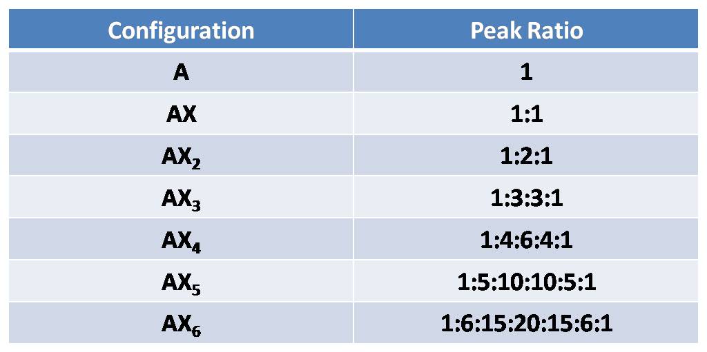
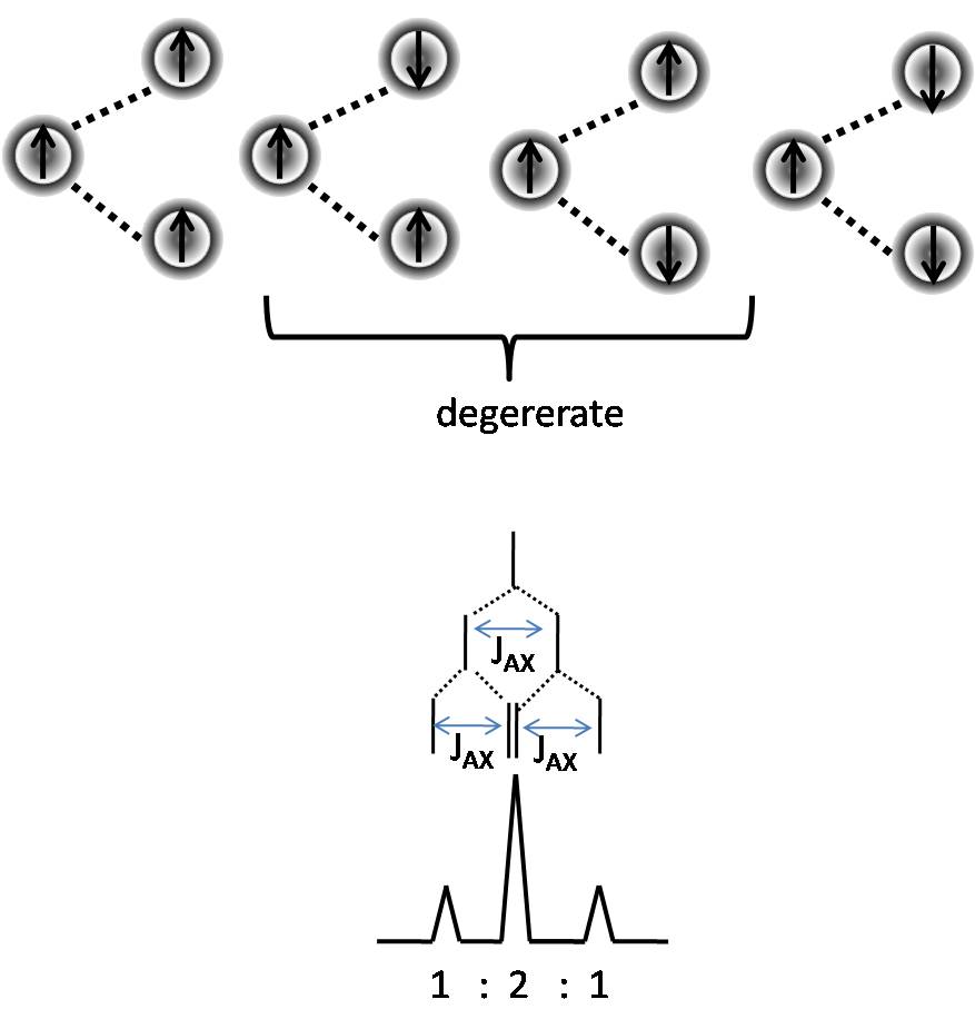
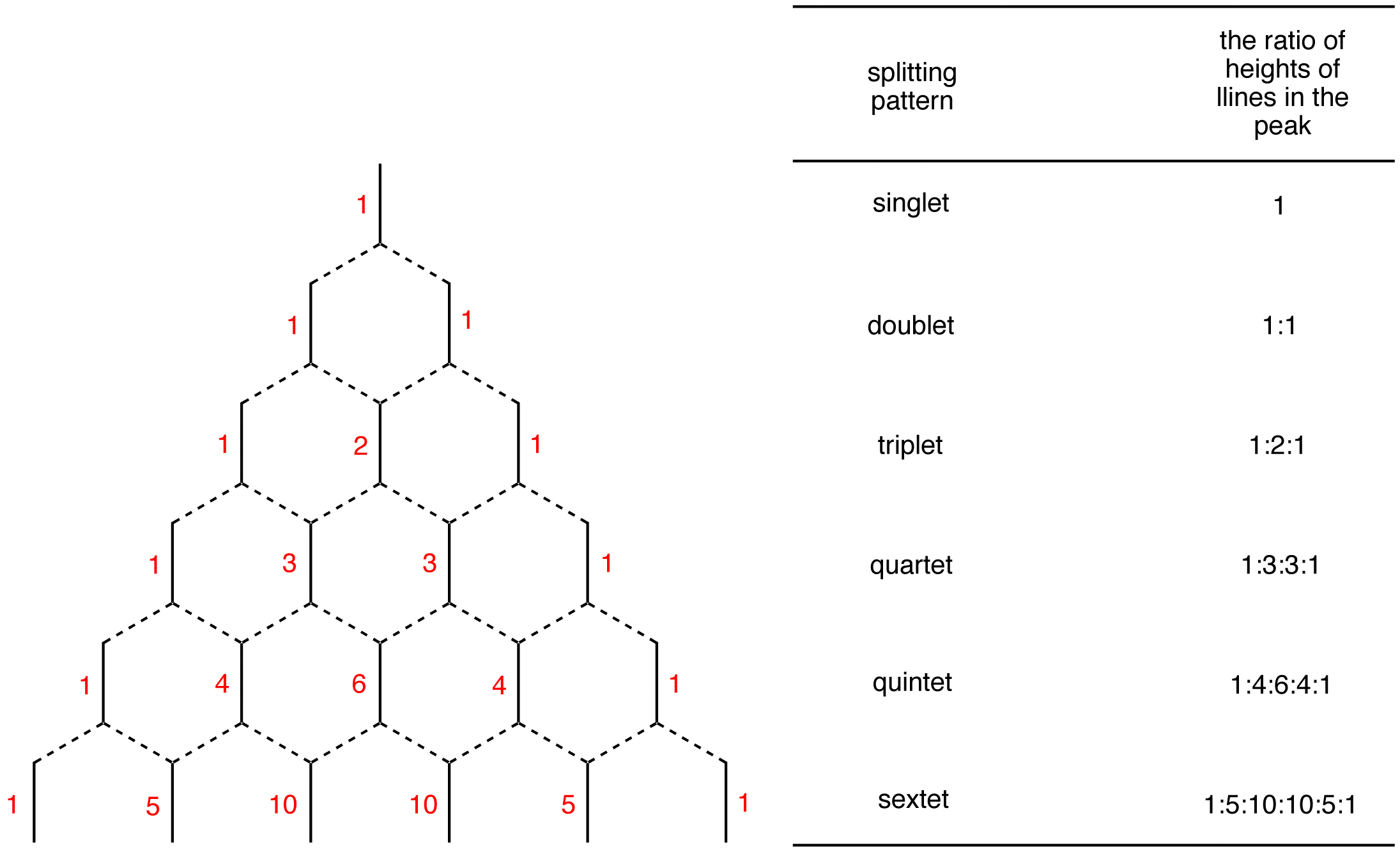
Nuclei in different chemical environments up to nine bonds (though 1-4 are typically readily measurable) is away can influence one another’s effective local magnetic field by carrying spin orientational information through bonding electrons.This effect is most prominent among chemically equivalent nuclei, giving rise to the N+1 rule for equivalent protons. A proton with N protons on contiguous carbon atoms splits into N+1 peaks with intensity pattern. The splitting pattern for A when it is coupled to a number of X nuclides would follow the relation represented by Pascal’s triangle. To be more specific, I will take AX2 for example. AX2 represent a spin system that contains three nuclei, two of which have the same chemical shift and one of which is different (e.g. ClCH2CHCl2). Here A is CH proton and X are CH2 protons. According to table 4 and figure 12, CH proton will be split into 1:1 doublet, while CH2 will give a fine structure of 1:2:1 triplet. The spacing between peaks is defined as coupling constant J, which can be used to describe the degree of coupling.
Table 4. Pascal's triangle according to AX configurations
Pascals Trinagle Construction
The Pascal’s triangle is a graphical device used to predict the ratio of heights of lines in a split NMR peak. To construct the Pascal’s triangle, use the following procedure.
Step 1: Draw a short, vertical line and write number one next to it.
![]()
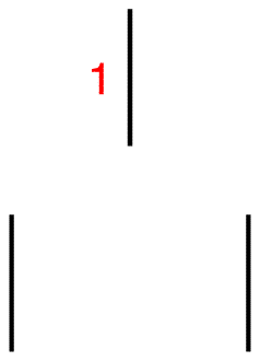
Step 2: Draw two vertical lines underneath it symmetrically.
Step 3: Connect each of them to the line above using broken lines.
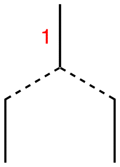
Step 4: Each of the two lines is connected to the single line above, which carries the number one. Therefore, write number one next to each line.
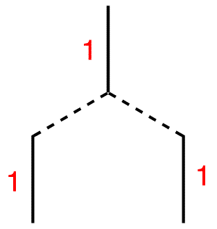
Step 5: Draw three vertical lines symmetrically underneath the two lines.
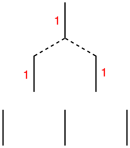
Step 6: Connect each of them to the nearest line(s) above.
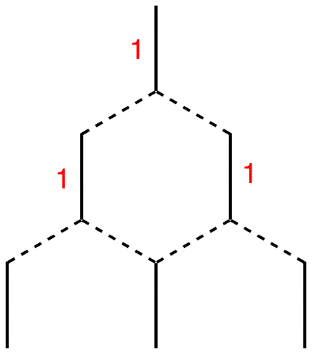
Step 7: Each terminal line is connected to one line above, which carries the number one. Therefore, write number one next to each of them. The internal line is connected to two lines above, each carrying the number one. 1 + 1 = 2; write number two next to the internal line.
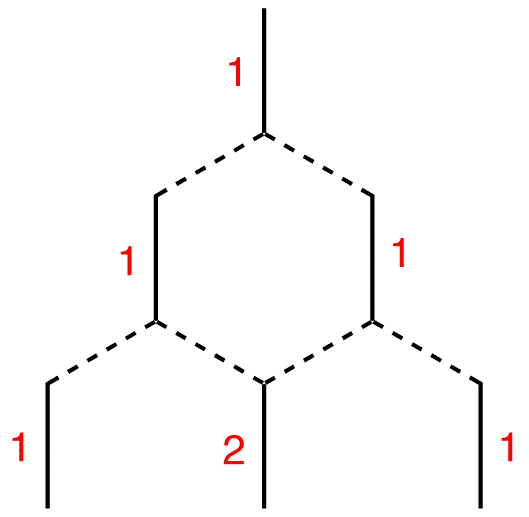
Continue the process as far down as necessary.
- see also (n+1) Rule, coupling constant
Strong Coupling and the Roof Effect
In the high field approximation, there may be strong coupling between homonuclear spins. Strong coupling refers to the scenario when the chemical shift difference (in Hz) is on the order of the J-coupling. As chemical shift scales with the magnetic field, the chemical shift differences are therefore smaller at low magnetic fields, makes this scenario more likely at low magnetic fields. First we must define the strong coupling parameter ,\(\theta\)
\[tan 2 \theta=\dfrac{2 \pi J}{\omega_A-\omega_B}\]
where \(\omega\) is in radians and J is in Hz.
[insert tan 2theta graph]
Then the J-coupling line intensities become for the doublet (A1,A2)
\[I_{A1} \propto 1-sin 2 \theta\]
\[I_{A2} \propto 1+sin 2 \theta\]
Just like with the usual J-couplings, having multiple J-couplings will lead to a complex splitting pattern, where each intensity is modified by the angle as such.
Expansion of the J-Coupling Hamiltonian
Typically, the J-coupling is given in the weak coupling limit. The weak coupling limit is defined by having \(\nu_I-\nu_s>>J\), which is typically valid at high magnetic fields of several tesla. However, here we will derive the J-coupling Hamiltonian for a 2 spin system without any assumptions about the coupling limit.
First we begin with the J-coupling Hamiltonian which constains the pertenent interactions; Zeeman and Scalar. Then the Hamiltonian will be
\(\omega_II_Z+\omega_SS_Z+2\pi J \textbf(I \cdot S)\)
The factor 2\(\pi\) in front of the J-coupling keeps all units in angular frequency, as J is measurable in Hz. Remember that for a 2 spin system, each nucleus has an \(\alpha\) and \(\beta\) state. Thus the potential wave functions in matrix form are given by the \(\alpha\) and \(\beta\) states. In Matrix form this would be represented for a 2 spin system as
\[\begin{bmatrix} |\alpha \alpha> & |\alpha \beta> \\ |\beta \alpha> & |\beta \beta> \end{bmatrix}\]
Now the \(\alpha\) and \(beta\) states also have matrix representations as
\[|\alpha>=\begin{bmatrix} 1\\0 \end{bmatrix}\]
\[|\beta>=\begin{bmatrix} 0\\1 \end{bmatrix}\]
and the combined states are given by cross product of the 2 matricies so
\[|\alpha\alpha>=\begin{bmatrix} 1\\0 \end{bmatrix} \times \begin{bmatrix} 1\\0 \end{bmatrix}=\begin{bmatrix} 1\\0\\0\\0\end{bmatrix}\]
\[|\beta\beta>=\begin{bmatrix} 0\\1 \end{bmatrix} \times \begin{bmatrix} 0\\1 \end{bmatrix}=\begin{bmatrix} 0\\0\\0\\1 \end{bmatrix}\]
\[|\alpha\beta>=\begin{bmatrix} 1\\0 \end{bmatrix} \times \begin{bmatrix} 0\\1 \end{bmatrix}=\begin{bmatrix} 0\\1\\0\\0 \end{bmatrix}\]
\[|\beta\alpha>=\begin{bmatrix} 0\\1 \end{bmatrix} \times \begin{bmatrix} 1\\0 \end{bmatrix}=\begin{bmatrix} 0\\0\\1\\0 \end{bmatrix}\]
Then without further proof (at the moment) the eigenfunctions of the 2 spin system are
\[\psi_1=|\alpha\alpha>\]
\[\psi_4=cos\theta|\alpha\beta>+sin\theta|\beta\alpha>\]
\[\psi_3=cos\theta|\beta\alpha>-sin\theta|\alpha\beta>\]
\[\psi_4=|\beta\beta>\]
Remember that according to Schroedinger's Equation,
\[\hat{H} \psi= E \psi\]
thus if we apply the Hamiltonian Operator on each of the eigenstates, we should be able to deduce the energy level. Now looking at the Hamiltonian, there are I and S operators which have the following matrix representations
\[I_z=S_z=\dfrac{1}{2}\begin{bmatrix} 1&0\\0&-1\end{bmatrix}\]
\[I_x=S_x=\dfrac{1}{2}\begin{bmatrix} 0&1\\1&0\end{bmatrix}\]
\[I_y=S_y=\dfrac{i}{2}\begin{bmatrix} 0&-1\\1&0\end{bmatrix}\]
However since we are considering a 2 spin system, 2x2 matrices won't cut it. Rather, we need to transform these matrices into the product basis by calculating the direct products of the wavefunctions. To do this we recognize that we can obtain 2N, wavefunctions where N is the total number of spins. To do this
\[\psi_k=|m_1> \times |m_2> ... \times |m_N>\]
Thus for \psi_1
\(\omega_II_Z+\omega_SS_Z+2\pi J \textbf(I \cdot S)\)
Limits of J-Couplings
There exists certain limits in which the J-coupling can be calculated. We begin our discussion investigating 13C-labeled methanol (13C-MeOH). Lets assume that we are in the high-temperature regime, such that the OH proton is uncoupled to the methyl spins during the experimental timescale. The J-coupling between the 3 methyl protons and the 13C nucleus is 1JHC=140.5 Hz.
High Field Limit
At high magnetic fields, the line width is governed by the magnetic field inhomogeneity. That is when a superconducting magnet is build, the field is not completely uniform over the sample volume. Therefore, there is a distribution of chemical shifts for a given site. Since the field inhomogeneity is typically small, (parts per billion or ppb), this leads to a broader peak than a perfectly homogenous field. This is the reason in which shimming is performed prior to sample collection. Shimming makes the field more homogenous. If we assume that the magnetic field inhomogeneity (Binhomo) of the external magnetic field (B0), is 25 ppb over the sample volume after shimming, then we can calculate the line width \(\Delta \nu\) of a single peak.
\( \Delta \nu =B_{0} B_{inhomo}\)
Assuming B0 is 11.74T (500 MHz spectrometer), then \(\Delta \nu\) is 2.1 Hz (~0.3 ppm). Of course there are geometrical constraints about the magnetic field inhomogenity, such as the fraction of sample that is in the inhomogenous region, but for now we assume that the equal portions of the sample are in the inhomogenous field. Thusly, J-couplings larger than 3.45 Hz could not be resolved. Of course this is ridiculous for a 500 MHz instrument with good shimming. A much more reasonable


Figure x: Magnitude of J-coupling that is un-resolvable J-couplings as a function of magnetic field, assuming a Binhomo=1.5 ppb. The regions of couplings that are resolvable are marked. Note that this assumes 1H
value would be not resolving J-couplings less than 0.2 H, which would be a field inhomogeneity of 0.10 ppb. Currently, the largest sustained magnetic fields are on the order of 100T (pulsed, National High Magnetic Field Lab) and ~30T (static). Therefore, the high field limit (\B_{HF}) can be described as
\(B_{HF}=J/(B_0 \Delta \nu \gamma)\)
or
\(B_{HF}=J/(B_0^2 B_{inhomo} \gamma)\)
where \(\gamma\) is the gyromagnetic ratio in Mhz/T and \(\Delta \nu\) is in ppm.
Thus, for the same field inhomogenity, the resolvable J-couplings are smaller for small \(\gamma\) nuclei.
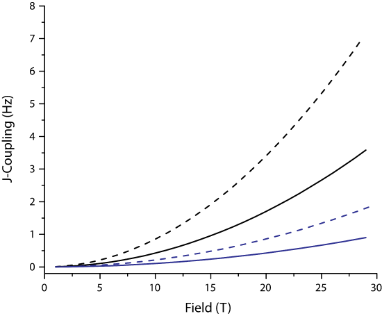
Figure x. Resolvable J-couplings for 1H (black) and 13C (blue) for \(\Delta \nu\) of 1.0 ppb (solid) and 2.0 ppb (dashed)
High Field Weak Coupling Limit
When the magnetic field is less than BHF, the heteronuclear J-couplings can be resolved. This leads to the well-known (2I+1) multiplet splitting. For spin I=1/2 (i.e. 1H, 13C, 31P) this leads to the well known pascal triangle. However, for coupling to spins I>1/2 (i.e. 14N, 2H, 7Li, 51V) the splitting patterns become more complex. As the J<<\(\nu\) we are in the weak coupling limit.
Low Field Strong Coupling Limit
\(B_{1 \rightarrow 2}^{Low Field}=\dfrac{J^2}{2 \Delta \nu (\gamma_I - \gamma_S)}\) First order Perturbation
\(B_{2 \rightarrow 3}^{Low Field}=\sqrt{\dfrac{3J^2}{4 \Delta \nu (\gamma_I - \gamma_S)^2}}\)
\(B_{3 \rightarrow exact}^{Low Field}=\dfrac{(1+\dfrac{1}{\sqrt{2}})J}{(\gamma_I - \gamma_S)}\)
Ultra Low Field Strong Coupling Limit
\(B_{exact \rightarrow 2}^{Ultra-Low Field}=\dfrac{4J}{(7\gamma_I - \gamma_S)}\)
Ultra-Low Field Weak Coupling Limit
\(B_{2 \rightarrow 1}^{Ultra-Low Field}=\sqrt{\dfrac{2 \Delta \nu J}{ (\gamma_I - \gamma_S)^2}}\)
Zero Field Weak Coupling Limit
\(B_{1 \rightarrow 0}^{Zero Field}=\dfrac{2 \Delta \nu J}{ (\gamma_I + \gamma_S)}\)
Outside Links
- This is not meant for references used for constructing the module, but as secondary and unvetted information available at other site
- Link to outside sources. Wikipedia entries should probably be referenced here.
Problems
1) Calculate the multiplicity for CH3 for both C and H.
2) Calculate the multiplicity for HCl for both H and Cl.
Contributors and Attributions
- Derrick Kaseman,
- Gamini Gunawardena from the OChemPal site (Utah Valley University)


