
1.9: Diffusion
- Page ID
- 408550

\( \newcommand{\vecs}[1]{\overset { \scriptstyle \rightharpoonup} {\mathbf{#1}} } \)
\( \newcommand{\vecd}[1]{\overset{-\!-\!\rightharpoonup}{\vphantom{a}\smash {#1}}} \)
\( \newcommand{\dsum}{\displaystyle\sum\limits} \)
\( \newcommand{\dint}{\displaystyle\int\limits} \)
\( \newcommand{\dlim}{\displaystyle\lim\limits} \)
\( \newcommand{\id}{\mathrm{id}}\) \( \newcommand{\Span}{\mathrm{span}}\)
( \newcommand{\kernel}{\mathrm{null}\,}\) \( \newcommand{\range}{\mathrm{range}\,}\)
\( \newcommand{\RealPart}{\mathrm{Re}}\) \( \newcommand{\ImaginaryPart}{\mathrm{Im}}\)
\( \newcommand{\Argument}{\mathrm{Arg}}\) \( \newcommand{\norm}[1]{\| #1 \|}\)
\( \newcommand{\inner}[2]{\langle #1, #2 \rangle}\)
\( \newcommand{\Span}{\mathrm{span}}\)
\( \newcommand{\id}{\mathrm{id}}\)
\( \newcommand{\Span}{\mathrm{span}}\)
\( \newcommand{\kernel}{\mathrm{null}\,}\)
\( \newcommand{\range}{\mathrm{range}\,}\)
\( \newcommand{\RealPart}{\mathrm{Re}}\)
\( \newcommand{\ImaginaryPart}{\mathrm{Im}}\)
\( \newcommand{\Argument}{\mathrm{Arg}}\)
\( \newcommand{\norm}[1]{\| #1 \|}\)
\( \newcommand{\inner}[2]{\langle #1, #2 \rangle}\)
\( \newcommand{\Span}{\mathrm{span}}\) \( \newcommand{\AA}{\unicode[.8,0]{x212B}}\)
\( \newcommand{\vectorA}[1]{\vec{#1}} % arrow\)
\( \newcommand{\vectorAt}[1]{\vec{\text{#1}}} % arrow\)
\( \newcommand{\vectorB}[1]{\overset { \scriptstyle \rightharpoonup} {\mathbf{#1}} } \)
\( \newcommand{\vectorC}[1]{\textbf{#1}} \)
\( \newcommand{\vectorD}[1]{\overrightarrow{#1}} \)
\( \newcommand{\vectorDt}[1]{\overrightarrow{\text{#1}}} \)
\( \newcommand{\vectE}[1]{\overset{-\!-\!\rightharpoonup}{\vphantom{a}\smash{\mathbf {#1}}}} \)
\( \newcommand{\vecs}[1]{\overset { \scriptstyle \rightharpoonup} {\mathbf{#1}} } \)
\(\newcommand{\longvect}{\overrightarrow}\)
\( \newcommand{\vecd}[1]{\overset{-\!-\!\rightharpoonup}{\vphantom{a}\smash {#1}}} \)
\(\newcommand{\avec}{\mathbf a}\) \(\newcommand{\bvec}{\mathbf b}\) \(\newcommand{\cvec}{\mathbf c}\) \(\newcommand{\dvec}{\mathbf d}\) \(\newcommand{\dtil}{\widetilde{\mathbf d}}\) \(\newcommand{\evec}{\mathbf e}\) \(\newcommand{\fvec}{\mathbf f}\) \(\newcommand{\nvec}{\mathbf n}\) \(\newcommand{\pvec}{\mathbf p}\) \(\newcommand{\qvec}{\mathbf q}\) \(\newcommand{\svec}{\mathbf s}\) \(\newcommand{\tvec}{\mathbf t}\) \(\newcommand{\uvec}{\mathbf u}\) \(\newcommand{\vvec}{\mathbf v}\) \(\newcommand{\wvec}{\mathbf w}\) \(\newcommand{\xvec}{\mathbf x}\) \(\newcommand{\yvec}{\mathbf y}\) \(\newcommand{\zvec}{\mathbf z}\) \(\newcommand{\rvec}{\mathbf r}\) \(\newcommand{\mvec}{\mathbf m}\) \(\newcommand{\zerovec}{\mathbf 0}\) \(\newcommand{\onevec}{\mathbf 1}\) \(\newcommand{\real}{\mathbb R}\) \(\newcommand{\twovec}[2]{\left[\begin{array}{r}#1 \\ #2 \end{array}\right]}\) \(\newcommand{\ctwovec}[2]{\left[\begin{array}{c}#1 \\ #2 \end{array}\right]}\) \(\newcommand{\threevec}[3]{\left[\begin{array}{r}#1 \\ #2 \\ #3 \end{array}\right]}\) \(\newcommand{\cthreevec}[3]{\left[\begin{array}{c}#1 \\ #2 \\ #3 \end{array}\right]}\) \(\newcommand{\fourvec}[4]{\left[\begin{array}{r}#1 \\ #2 \\ #3 \\ #4 \end{array}\right]}\) \(\newcommand{\cfourvec}[4]{\left[\begin{array}{c}#1 \\ #2 \\ #3 \\ #4 \end{array}\right]}\) \(\newcommand{\fivevec}[5]{\left[\begin{array}{r}#1 \\ #2 \\ #3 \\ #4 \\ #5 \\ \end{array}\right]}\) \(\newcommand{\cfivevec}[5]{\left[\begin{array}{c}#1 \\ #2 \\ #3 \\ #4 \\ #5 \\ \end{array}\right]}\) \(\newcommand{\mattwo}[4]{\left[\begin{array}{rr}#1 \amp #2 \\ #3 \amp #4 \\ \end{array}\right]}\) \(\newcommand{\laspan}[1]{\text{Span}\{#1\}}\) \(\newcommand{\bcal}{\cal B}\) \(\newcommand{\ccal}{\cal C}\) \(\newcommand{\scal}{\cal S}\) \(\newcommand{\wcal}{\cal W}\) \(\newcommand{\ecal}{\cal E}\) \(\newcommand{\coords}[2]{\left\{#1\right\}_{#2}}\) \(\newcommand{\gray}[1]{\color{gray}{#1}}\) \(\newcommand{\lgray}[1]{\color{lightgray}{#1}}\) \(\newcommand{\rank}{\operatorname{rank}}\) \(\newcommand{\row}{\text{Row}}\) \(\newcommand{\col}{\text{Col}}\) \(\renewcommand{\row}{\text{Row}}\) \(\newcommand{\nul}{\text{Nul}}\) \(\newcommand{\var}{\text{Var}}\) \(\newcommand{\corr}{\text{corr}}\) \(\newcommand{\len}[1]{\left|#1\right|}\) \(\newcommand{\bbar}{\overline{\bvec}}\) \(\newcommand{\bhat}{\widehat{\bvec}}\) \(\newcommand{\bperp}{\bvec^\perp}\) \(\newcommand{\xhat}{\widehat{\xvec}}\) \(\newcommand{\vhat}{\widehat{\vvec}}\) \(\newcommand{\uhat}{\widehat{\uvec}}\) \(\newcommand{\what}{\widehat{\wvec}}\) \(\newcommand{\Sighat}{\widehat{\Sigma}}\) \(\newcommand{\lt}{<}\) \(\newcommand{\gt}{>}\) \(\newcommand{\amp}{&}\) \(\definecolor{fillinmathshade}{gray}{0.9}\)1. DIFFUSION
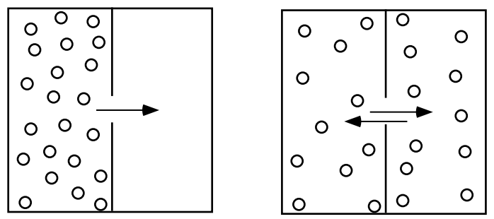
At any temperature different from absolute zero all atoms, irrespective of their state of aggregation (gaseous, liquid or solid), are constantly in motion. Since the movement of particles is associated with collisions, the path of a single particle is a zigzag one. However, an aggregation of “diffusing” particles has an observable drift from places of higher to places of lower concentration (fig. 1). For this reason diffusion is known as a transport phenomenon.
In each diffusion reaction (heat flow, for example, is also a diffusion process), the flux (of matter, heat, electricity, etc.) follows the general relation:
Flux = (conductivity) x (driving force)
In the case of atomic or molecular diffusion, the “conductivity” is referred to as the diffusivity or the diffusion constant, and is represented by the symbol D. We realize from the above considerations that this diffusion constant (D) reflects the mobility of the diffusing species in the given environment and accordingly assumes larger values in gases, smaller ones in liquids, and extremely small ones in solids.
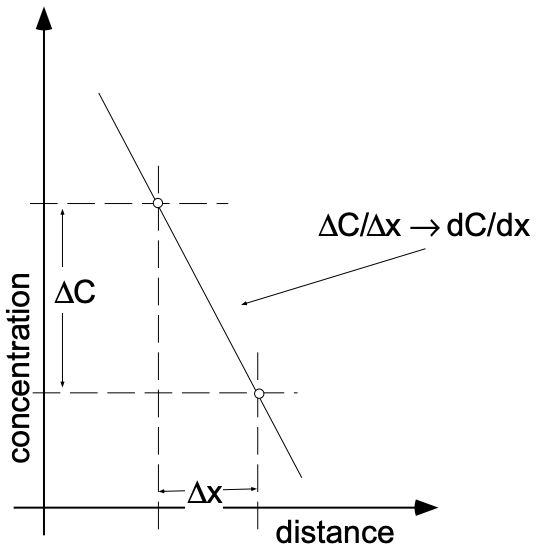
The “driving force” for many types of diffusion is the existence of a concentration gradient. The term “gradient” describes the variation of a given property as a function of distance in the x-direction. If a material exhibits a linear variation of concentration with distance in the x-direction, we speak of a constant concentration gradient in the x-direction. The gradient itself is the rate of change of the concentration with distance (dc/dx), which is the same as the slope of a graph of concentration vs. position (\(\Delta c/\Delta x)\) (see fig. 2).
Steady State and Nonsteady Diffusion
Diffusion processes may be divided into two types: (a) steady state and (b) nonsteady state. Steady state diffusion takes place at a constant rate - that is, once the process starts the number of atoms (or moles) crossing a given interface (the flux) is constant with time. This means that throughout the system dc/dx = constant and dc/dt = 0.
Nonsteady state diffusion is a time dependent process in which the rate of diffusion is a function of time. Thus dc/dx varies with time and dc/dt ≠ 0. Both types of diffusion are described quantitatively by Fick’s laws of diffusion. The first law concerns both steady state and nonsteady state diffusion, while the second law deals only with nonsteady state diffusion.
2. STEADY STATE DIFFUSION (FICK’S FIRST LAW)
On the basis of the above considerations, Fick’s First Law may be formulated as:
\(\mathrm{J}=-\mathrm{D}\left(\dfrac{\mathrm{dc}}{\mathrm{dx}}\right)\) In words: The diffusive flux is proportional to the existing concentration gradient.
The negative sign in this relationship indicates that particle flow occurs in a "down" gradient direction, i.e. from regions of higher to regions of lower concentration. The flux \(\mathrm{J}\) can be given in units of atoms \(/ \mathrm{cm}^2 \mathrm{~s}\), moles/ \(\mathrm{cm}^2 \mathrm{~s}\), or equivalents. Correspondingly, the diffusivity (D) will assume the dimensions \(\mathrm{cm}^2 / \mathrm{s}\), as can be seen from a dimensional analysis:
\(\mathrm{J}\left(\dfrac{\text { moles }}{\mathrm{cm}^2 \mathrm{~s}}\right)=-\mathrm{D}\left(\dfrac{\mathrm{dc}}{\mathrm{dx}}\right)\left(\dfrac{\text { moles } \cdot \mathrm{cm}^{-3}}{\mathrm{~cm}}\right)\)
Thus: \(D=\mathrm{cm}^2 / \mathrm{s}\)
Like chemical reactions, diffusion is a thermally activated process and the temperature dependence of diffusion appears in the diffusivity as an “Arrhenius-type” equation:
\(D=D_0 e^{-E_a / R T}\)
where \(D_o\) (the equivalent of \(A\) in the previously discussed temperature dependence of the rate constant) includes such factors as the jump distance, the vibrational frequency of the diffusing species and so on. Selected values of \(D, D_0\) and \(E_a\) are given in Table 1 (a) and (b).
TABLE 1
(a) Selected Values of Diffusion Constants (D)
\begin{aligned}
&\begin{array}{llrl}
\underline{\text { Diffusing Substance }} & \underline{\text { Solvent }} & \underline{T\left({ }^{\circ} \mathrm{C}\right)} & \underline{D\left(\mathrm{~cm}^2 \cdot \mathrm{s}^{-1}\right)} \\
\mathrm{Au} & \mathrm{Cu} & 400 & 5 \times 10^{-13} \\
\mathrm{Cu} \text { (Self-Diffusing) } & (\mathrm{Cu}) & 650 & 3.2 \times 10^{-12} \\
\mathrm{C} & \mathrm{Fe} \text { (FCC) } & 950 & 10^{-7} \\
\text { Methanol } & \mathrm{H}_2 \mathrm{O} & 18 & 1.4 \times 10^{-5} \\
\mathrm{O}_2 & \text { Air } & 0 & 0.178 \\
\mathrm{H}_2 & \text { Air } & 0 & 0.611
\end{array}\\
\end{aligned}
| Solute | Solvent (host structure) | \(\underline{D_o, \mathrm{cm}^2 \mathrm{s}}\) | \(\underline{E_a}\), kJoules/mole |
|---|---|---|---|
| 1. Carbon | fcc iron | 0.2100 | 142 |
| 2. Carbon | bcc iron | 0.0079 | 76 |
| 3. Iron | fcc iron | 0.5800 | 185 |
| 4. Iron | bcc iron | 5.8000 | 251 |
| 5. Nickel | fcc iron | 0.5000 | 276 |
| 6. Manganese | fcc iron | 0.3500 | 283 |
| 7. Zinc | copper | 0.0330 | 159 |
| 8. Copper | aluminum | 2.0000 | 142 |
| 9. Copper | copper | 11.0000 | 240 |
| 10. Silver | silver | 0.7200 | 188 |
A typical application of Fick's first law: Determine the rate at which helium (He), held at 5 atm and \(200^{\circ} \mathrm{C}\) in a Pyrex glass bulb of \(50 \mathrm{~cm}\) diameter and a wall thickness ( \(\mathrm{x}\) ) of \(0.1 \mathrm{~cm}\), diffuses through the Pyrex to the outside. Assume that the pressure outside the tube at all times remains negligible (see fig. 3). (For the diffusion of gases it is

customary, although not necessary, to replace the diffusion constant \(D\) with the Permeation constant \(\mathrm{K}\), normally given in units of \(\mathrm{cm}^2 / \mathrm{s} \cdot\) atm. Using the gas laws, \(\mathrm{K}\) is readily converted to \(\mathrm{D}\) if so desired.)
In the present system
\(\mathrm{K}=1 \times 10^{-9} \mathrm{~cm}^2 / \mathrm{s} \cdot \mathrm{atm}\)
We can now set up the diffusion equation:
\(J=-\mathrm{K}\left(\frac{\mathrm{dP}}{\mathrm{dx}}\right) \quad \begin{aligned}
&\text { (and operate with pressures instead } \\
&\text { of concentrations) }
\end{aligned}\)
We may now formally separate the variables and integrate:
\begin{aligned}
J \mathrm{dx} &=-\mathrm{KdP} \\
\int_{\mathrm{x}=0}^{\mathrm{x}=0.1} \mathrm{Jdx} &=-\int_{\mathrm{p}_2=5}^{p_1=0} \mathrm{KdP} \\
\mathrm{J} &=\mathrm{K} \frac{5.0}{0.1}
\end{aligned}
We can forego the integration since \((\mathrm{dP} / \mathrm{dx})=(\Delta \mathrm{P} / \Delta \mathrm{x})\) and we may immediately write:
\begin{aligned}
\mathrm{J}(\text { total }) &=-\mathrm{K} \frac{\Delta \mathrm{P}}{\Delta \mathrm{x}} \times \mathrm{A}=5 \times 10^{-8} \times 7.9 \times 10^3 \\
\mathrm{~J} &=3.9 \times 10^{-4} ? ?
\end{aligned}
The units of the flux may be obtained from a dimensional analysis:
\(\mathrm{J}=-\mathrm{K} \times \dfrac{\Delta \mathrm{P}}{\Delta \mathrm{x}} \times \mathrm{A}=\dfrac{\mathrm{cm}^2}{\mathrm{~s} \cdot \mathrm{atm}} \dfrac{\mathrm{atm}}{\mathrm{cm}} \dfrac{\mathrm{cm}^2}{1}=\dfrac{\mathrm{cm}^3}{\mathrm{~s}}\)
The total flux is \(3.9 \times 10^{-4} \mathrm{~cm}^3 / \mathrm{s}\) (with the gas volume given for \(0^{\circ} \mathrm{C}\) and \(1 \mathrm{~atm}\) ). If the total gas flow by diffusion were to be determined for a specified time interval, the volume would be multiplied by the indicated time.
3. NONSTEADY STATE DIFFUSION (FICK’S SECOND LAW)
The quantitative treatment of nonsteady state diffusion processes is formulated as a partial differential equation. It is beyond the scope of 3.091 to treat the equations in detail but we can consider the second law qualitatively and examine some relevant solutions quantitatively.
The difference between steady state and nonsteady state diffusion conditions can readily be visualized (fig. 4). In the first case we have, for example, the diffusion of gas
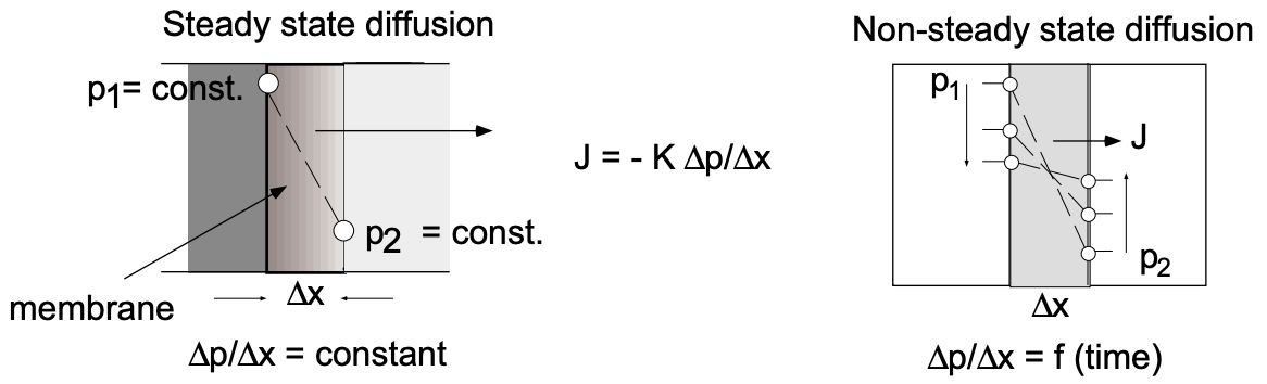
from an infinite volume (\(\mathrm{P}_1\) const) through a membrane into an infinite volume (\(\mathrm{P}_2\) const). The pressure gradient across the membrane remains constant as does the diffusive flux. In the second case we deal with diffusion from a finite volume through a membrane into a finite volume. The pressures in the reservoirs involved change with time as does, consequently, the pressure gradient across the membrane.
(You are not required to be familiar with the following derivation of the Second Fick’s Law, but you must know its final form.)
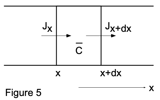
Consider a volume element (between x and x+dx of unit cross sectional area) of a membrane separating two finite volumes involved in a diffusion system (fig. 5). The flux of a given material into the volume element minus the flux out of the volume element equals the rate of accumulation of the material into this volume element:
\(J_x-J_{x+d x}=\dfrac{\partial \bar{c}}{\partial t} d x\)
[ \(\bar{c}\) is the average concentration in the volume element and \(\bar{c} d x\) is the total amount of the diffusing material in the element at time (t).]
Using a Taylor series we can expand \(J_{x+d x}\) about \(x\) and obtain:
\(J_{x+d x}=J_x+\dfrac{\partial J_x}{\partial x} d x+\dfrac{\partial^2 J_x}{\partial x^2} \dfrac{d x^2}{2}+\ldots\)
Accordingly, as \(\mathrm{dx} \rightarrow 0\):
\(\dfrac{\partial}{\partial x}\left(D \dfrac{\partial c}{d x}\right)=\dfrac{\partial c}{\partial t}\)
and if \(D\) does not vary with \(x\) (which is normally the case) we have the formulation of Fick's Second Law:
\(\dfrac{\partial \mathrm{C}}{\partial \mathrm{t}}=\mathrm{D} \dfrac{\partial^2 \mathrm{C}}{\partial \mathrm{x}^2} \quad \text { (Fick's Second Law) }\)
In physical terms this relationship states that the rate of compositional change is proportional to the “rate of change” of the concentration gradient rather than to the concentration gradient itself.
The solutions to Fick’s second law depend on the boundary conditions imposed by the particular problem of interest. As an example, let us consider the following problem (encountered in many solid state processes):
A frequently encountered situation is the diffusion of a component 2 into an infinite region of a material 1 (fig. 6) [planar diffusion of doping elements into semiconductors
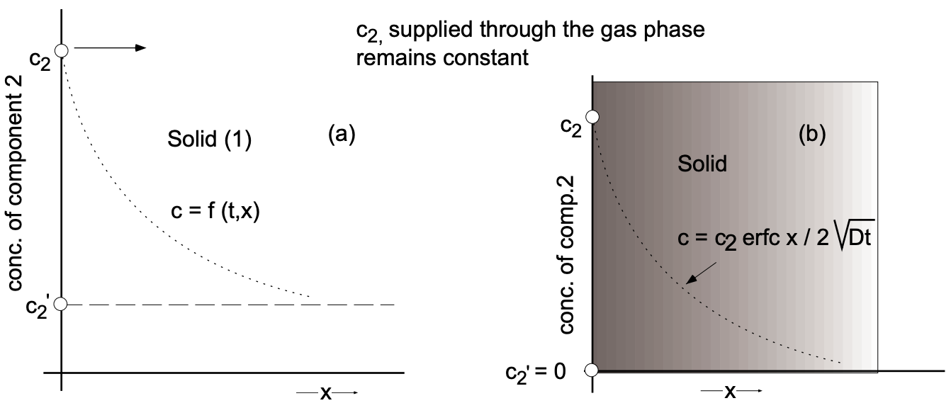
for the generation of junction devices (p-n junctions, junction transistors)]. The boundary conditions are: the concentration of component (2) at the surface of the solid phase \((x=0)\) remains constant at \(c_2\) and the concentration of component (2) in the solid prior to diffusion is uniformly \(c_{2^{\prime}}\) (a). Under these boundary conditions the solution to Fick's second law assumes the form:
\(\dfrac{c_2-c}{c_2-c_{2^{\prime}}}=\operatorname{erf}\left(\dfrac{x}{2 \sqrt{D t}}\right)\)
If no component (2) is originally in the solid matrix (1) (b), the above solution is simpler:
\begin{aligned}
\dfrac{c_2-c}{c_2} &=\operatorname{erf}\left(\dfrac{x}{2 \sqrt{D t}}\right) \\
1-\dfrac{c}{c_2} &=\operatorname{erf}\left(\dfrac{x}{2 \sqrt{D t}}\right) \\
\dfrac{c}{c_2} &=1-\operatorname{erf}\left(\dfrac{x}{2 \sqrt{D t}}\right) \\
\dfrac{c}{c_2} &=\operatorname{erfc}\left(\dfrac{x}{2 \sqrt{D t}}\right) \\
c &=c_2 \text { erfc }\left(\dfrac{x}{2 \sqrt{D t}}\right)
\end{aligned}
An analysis shows that the last form of the solution to Fick's law relates the concentration (c) at any position ( \(\mathrm{x}\) ) (depth of penetration into the solid matrix) and time (t) to the surface concentration \(\left(c_2\right)\) and the diffusion constant \((D)\). The terms erf and erfc stand for error function and complementary error function respectively - it is the Gaussian error function as tabulated (like trigonometric and exponential functions) in mathematical tables. Its limiting values are:
\begin{aligned}
&\text{erf}(0) &&= 0 \\
&\text{erf}(\infty) &&= 1 \quad &&\text{And for the complementary error function:} \\
&\text{erf}(-\infty) &&=-1 \quad &&\text{erfc = (1-erf)}
\end{aligned}
Another look at the above solution to the diffusion equation shows that the concentration (c) of component (2) in the solid is expressed in terms of the error function of the argument \(x / 2 \sqrt{D t}\). To determine at what depth a particular concentration \(\left(\mathrm{c}^*\right)\) of (2) will appear, we substitute this concentration for (c) and obtain:
\(\dfrac{c^*}{c_2}=\operatorname{erfc}\left(\dfrac{x}{2 \sqrt{D t}}\right)=K\)
Since the error function is a constant, its argument must also be a constant:
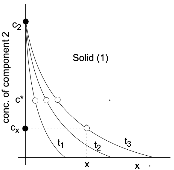
\(\dfrac{x}{2 \sqrt{D t}}=K^{\prime}\)
Therefore, under the given boundary conditions:
\begin{aligned}
&x=K^{\prime} 2 \sqrt{D t} \\
&x=K^{\prime} \cdot \sqrt{D t} \\
&x \propto \sqrt{t}
\end{aligned}
The depth of penetration of a specified concentration is found to be proportional to the square root of the time of diffusion.
4. SELF-DIFFUSION
As previously indicated, the thermal motion of atoms in a lattice is a random process and as such will lead to local displacements of individual atoms. This random movement of atoms within a lattice (self-diffusion), which is not associated with any existing concentration gradients, can be readily demonstrated with the aid of “radioactive elements”. For example, nickel appears in nature in the form of several “stable isotopes”:
\(\mathrm{Ni}_{28}^{58}, \mathrm{Ni}_{28}^{60}, \mathrm{Ni}_{28}^{61}, \mathrm{Ni}_{28}^{62}\) and \(\mathrm{Ni}_{28}^{64}\)
If \(\mathrm{Ni}_{28}^{58}\) is irradiated with neutrons in a nuclear reactor, it will capture a neutron and become \(\mathrm{Ni}_{28}^{59}\) which is radioactive (a radio-isotope).
\(\mathrm{Ni}_{28}^{58}+\mathrm{n} \rightarrow \mathrm{Ni}_{28}^{59} \rightarrow \mathrm{Co}_{27}^{59}+\gamma+\beta\)
Nickel 59 is characterized by its instability which leads to the emission of \(\beta\) and \(\gamma\) radiation, with a half-life of \(8 \times 10^4\) years. Since this radiation can be measured by appropriate radiation detectors, it is possible to use \(\mathrm{Ni}_{59}\) as a "tracer element" for studies of self-diffusion.
The radioactive nickel (which is identical to ordinary nickel with the exception of its radioactive properties) is electroplated onto normal nickel. This specimen is subsequently placed into a furnace and heated up to close to its melting point for an extended period of time. After removing the specimen, it is sectioned into slices parallel to the surface which contained the radioactive tracer element. With the aid of a radiation detector it can now be shown that the \(\mathrm{Ni}_{59}\), which originally was only at the surface, has diffused into the bulk material while simultaneously some bulk nickel has counter-diffused in the other direction. If this sample is heat-treated for a much longer time, sectioning and counting will reveal a completely uniform distribution of the radio-tracer element. It can thus be shown that self-diffusion does occur in solids, and quantitative measurements with tracer elements even permit the determination of self-diffusion coefficients.
5. DIFFUSION MECHANISMS
The diffusion process in interstitial solid solutions, like that of carbon in iron, can readily be understood as a result of considerable differences in atomic diameters. However, the fact that \(\mathrm{Au}\) diffuses faster in \(\mathrm{Pb}\) than \(\mathrm{NaCl}\) diffuses in water at \(15^{\circ} \mathrm{C}\) cannot be readily explained. The magnitude of the observed activation energy indicates that a mechanism whereby atoms simply change places with each other has to be excluded. More reasonable mechanisms were suggested by Frenkel and Schottky. They proposed the existence of point defects (vacancies) in crystals which provide a mechanism by which atoms can move (diffuse) within a crystal. The concentration of such vacancies, as you recall, can be calculated from simple statistical calculations.
In most solids we are not dealing with single crystals but rather with polycrystalline materials which contain a large number of grain boundaries (internal surfaces). As expected, the rate of diffusion along grain boundaries is much higher than that for volume diffusion ( \(D_{\text {volume }}<D_{\text {g-boundary }}\) ). Finally, surface diffusion, which takes place on all external surfaces, is even higher \(\left(D_{\text {volume }}<D_{\text {g-boundary }}<D_{\text {surface }}\right)\). The respective activation energies for diffusion are:
\(E_a\) surface \(<E_a\) grain boundary \(<E_a\) volume
Diffusion in Non-Metals
In non-metallic systems diffusion takes place by the same mechanisms as in metallic systems. Oxygen, for example, diffuses through many oxides by vacancy migration. In crystalline oxides and in silicate glasses as well, it is found that oxygen diffuses much more rapidly than the metallic ion. In glasses containing alkali atoms \(\left(\mathrm{Na}^{+}, \mathrm{K}^{+}\right)\), the respective rates of diffusion are:
\[D_{\text {alkali }}>D_{\text {oxygen }}>D_{\text {silicon }}\]
corresponding to differences in bonding strengths. In polymer materials diffusion requires the motion of large molecules since intramolecular bonding is much stronger than intermolecular bonding. This fact explains that the diffusion rates in such materials are relatively small.
Gaseous Diffusion in Solids
Some gases, like hydrogen and helium, diffuse through some metals with ease even at room temperature. Helium, for example, will diffuse through quartz and steel and limits the ultimate vacuum obtainable in ultra-high vacuum systems. Hydrogen similarly diffuses readily through \(\mathrm{Ni}\) at elevated temperatures. \(\mathrm{H}_2\) also diffuses at high rates through palladium - a phenomenon which is used extensively for hydrogen purification since that material is impervious to other gases.
| \(z\) | \(erf(z)\) | \(z\) | \(erf(z)\) |
|---|---|---|---|
| 0 | 0 | 0.85 | 0.7707 |
| 0.025 | 0.0282 | 0.90 | 0.7970 |
| 0.05 | 0.0564 | 0.95 | 0.8209 |
| 0.10 | 0.1125 | 1.0 | 0.8427 |
| 0.15 | 0.1680 | 1.1 | 0.8802 |
| 0.20 | 0.2227 | 1.2 | 0.9103 |
| 0.25 | 0.2763 | 1.3 | 0.9340 |
| 0.30 | 0.3286 | 1.4 | 0.9523 |
| 0.35 | 0.3794 | 1.5 | 0.9661 |
| 0.40 | 0.4234 | 1.6 | 0.9763 |
| 0.45 | 0.4755 | 1.7 | 0.9838 |
| 0.50 | 0.5205 | 1.8 | 0.9891 |
| 0.55 | 0.5633 | 1.9 | 0.9928 |
| 0.60 | 0.6039 | 2.0 | 0.9953 |
| 0.65 | 0.6420 | 2.2 | 0.9981 |
| 0.70 | 0.6778 | 2.4 | 0.9993 |
| 0.75 | 0.7112 | 2.6 | 0.9998 |
| 0.80 | 0.7421 | 2.8 | 0.9999 |
SOURCE: The values of erf(z) to 15 places, in increments of z of 0.0001, can be found in the Mathematical Tables Project, “Table of Probability Functions . . .”, vol. 1, Federal Works Agency, Works Projects Administration, New York, 1941. A discussion of the evaluation of erf(z), its derivatives and integrals, with a brief table is given by H. Carslaw and J. Jaeger, in Appendix 2 of “Conduction of Heat in Solids”, Oxford University Press, Fair Lawn, NJ, 1959.