1.10: Phase Equilibria and Phase Diagrams

PHASE EQUILIBRIA AND PHASE DIAGRAMS

Phase diagrams are one of the most important sources of information concerning the behavior of elements, compounds and solutions. They provide us with the knowledge of phase composition and phase stability as a function of temperature (T), pressure (P) and composition (C). Furthermore, they permit us to study and control important processes such as phase separation, solidification, sintering, purification, growth and doping of single crystals for technological and other applications. Although phase diagrams provide information about systems at equilibrium, they can also assist in predicting phase relations, compositional changes and structures in systems not at equilibrium.

GASES, LIQUIDS AND SOLIDS

Any material (elemental or compound) can exist as a gas, a liquid or a solid, depending on the relative magnitude of the attractive interatomic or intermolecular forces vs the disruptive thermal forces. It is thus clear that the stability (existence) of the different states of aggregation, which are referred to as phases, is a function of temperature and pressure (since with increased pressure the atoms, for exampled of a gas phase, are closer spaced and thus subject to increased interatomic attraction).

In general terms, a “phase” is a homogeneous, physically distinct, mechanically separable portion of a material with a given chemical composition. To illustrate this definition, let us look at a few examples of common multi-phase systems. Ice cubes in water constitute a two-phase system (ice and liquid water), unless we include the vapor above the glass in our system, which would make it a three-phase system. A mixture of oil and water would also be a two-phase system. Just as oil and water represent two distinct liquid phases, two regions of a solid with distinctly different composition or structure separated by boundaries represent two solid phases.

If we look at a one-component system, such as liquid water, we recognize that because of the energy distribution of the water molecules, some water molecules will always possess sufficient energy to overcome the attractive forces on the surface of \(\mathrm{H}_{2} \mathrm{O}\) and enter into the gas phase. If thermal energy is continuously supplied to a liquid in an open container, the supply of high energy molecules (which leave the liquid phase) is replenished and the temperature remains constant - otherwise the loss of high energy molecules will lower the temperature of the system. The total quantity of heat necessary to completely "vaporize" one mole of a liquid at its boiling point is called its molar heat of vaporization, designated by \(\Delta \mathrm{H}_{\mathrm{V}}\). Similarly, the heat required to completely melt one mole of a solid (the heat required to break the bonds established in the solid phase) is called the (latent) heat of fusion ( \(\Delta \mathrm{H}_{\mathrm{V}}\) ).

Visualize a liquid in a sealed container with some space above the liquid surface. Again, some of the most energetic liquid molecules will leave the liquid phase and form a "gas phase" above the liquid. Since gas molecules will thus accumulate in the gas phase (at a constant temperature), it is inevitable that as a result of collisions in the gas phase some molecules will re-enter the liquid phase and a situation will be established whereby the rate of evaporation will equal the rate of condensation – i.e., a dynamic equilibrium between the liquid and gas phase will exist. The established pressure in the gas phase is referred to as the equilibrium vapor pressure, which is normally significantly less for solids than for liquids.

For obvious reasons it is desirable to know for any given material the conditions (P, T) under which the solid state, the liquid state and the gaseous state are stable, as well as the conditions under which the solid and liquid phases may coexist. These conditions are graphically presented in equilibrium phase diagrams, which can be experimentally determined.

ONE-COMPONENT PHASE DIAGRAM

Figure 1 illustrates the temperatures and pressures at which water can exist as a solid, liquid or vapor. The curves represent the points at which two of the phases coexist in equilibrium. At the point \(T_{t}\) vapor, liquid and solid coexist in equilibrium. In the fields of the diagram (phase fields) only one phase exists. Although a diagram of this kind delineates the boundaries of the phase fields, it does not indicate the quantity of any phase present.

It is of interest to consider the slope of the liquid/solid phase line of the \(\mathrm{H}_{2} \mathrm{O}\) phase diagram. It can readily be seen that if ice \(-\) say at \(-2^{\circ} \mathrm{C}-\) is subjected to high pressures, it will transform to liquid \(\mathrm{H}_{2} \mathrm{O}\). (An ice skater will skate not on ice, but on water.) This particular pressure sensitivity (reflected in the slope of the solid/liquid phase line) is characteristic for materials which have a higher coordination number in the liquid than in the solid phase \(\left(\mathrm{H}_{2} \mathrm{O}, \mathrm{Bi}, \mathrm{Si}, \mathrm{Ge}\right)\). Metals, for example have an opposite slope of the solid/liquid phase line, and the liquid phase will condense under pressure to a solid phase.

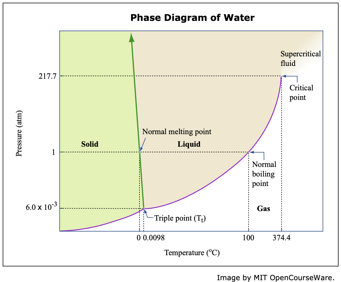
Fig. 1 Pressure/Temperature Diagram for Water. (Not drawn to scale.)

PHASE RULE AND EQUILIBRIUM

The phase rule, also known as the Gibbs phase rule, relates the number of components and the number of degrees of freedom in a system at equilibrium by the formula

\[F = C - P + 2 \tag{1}\]

where F equals the number of degrees of freedom or the number of independent variables, C equals the number of components in a system in equilibrium and P equals the number of phases. The digit 2 stands for the two variables, temperature and pressure.

\[\mathrm{CaCO}_{3}(\mathrm{~s}) \leftrightarrows \mathrm{CaO}(\mathrm{s})+\mathrm{CO}_{2}(\mathrm{~g}) \tag{2}\]

There are also three different chemical constituents, but the number of components is only two because any two constituents completely define the system in equilibrium. Any third constituent may be determined if the concentration of the other two is known. Substituting into the phase rule (eq. [1]) we can see that the system is univariant, since \(F=C-P+2=2-3+2=1\). Therefore only one variable, either temperature or pressure, can be changed independently. (The number of components is not always easy to determine at first glance, and it may require careful examination of the physical conditions of the system at equilibrium.)

The phase rule applies to dynamic and reversible processes where a system is heterogeneous and in equilibrium and where the only external variables are temperature, pressure and concentration. For one-component systems the maximum number of variables to be considered is two - pressure and temperature. Such systems can easily be represented graphically by ordinary rectangular coordinates. For two-component (or binary) systems the maximum number of variables is three pressure, temperature and concentration. Only one concentration is required to define the composition since the second component is found by subtracting from unity. A graphical representation of such a system requires a three-dimensional diagram. This, however, is not well suited to illustration and consequently separate two-coordinate diagrams, such as pressure vs temperature, pressure vs composition and temperature vs composition, are mostly used. Solid/liquid systems are usually investigated at constant pressure, and thus only two variables need to be considered – the vapor pressure for such systems can be neglected. This is called a condensed system and finds considerable application in studying phase equilibria in various engineering materials. A condensed system will be represented by the following modified phase rule equation:

\[F = C - P + 1 \tag{3}\]

where all symbols are the same as before, but (because of a constant pressure) the digit 2 is replaced by the digit 1, which stands for temperature as variable. The graphical representation of a solid/liquid binary system can be simplified by representing it on ordinary rectangular coordinates: temperature vs concentration or composition.

PHASE DIAGRAM

With the aid of a suitable calorimeter and energy reservoir, it is possible to measure the heat required to melt and evaporate a pure substance like ice. The experimental data obtainable for a mole of ice is shown schematically in fig. 2. As heat is added to the solid, the temperature rises along line "a" until the temperature of fusion \(\left(T_{f}\right)\) is reached. The amount of heat absorbed per mole during melting is represented by the length of line " \(\mathrm{b}\) ", or \(\Delta \mathrm{H}_{\mathrm{F}}\). The amount of heat absorbed per mole during evaporation at the boiling point is represented by line " \(d\) ". The reciprocal of the slope of line "a", \((d H / d T)\), is the heat required to change the temperature of one mole of substance (at constant pressure) by \(1^{\circ} \mathrm{CF} .(\mathrm{dH} / \mathrm{dT})\) is the molar heat capacity of a material, referred to as " \(\mathrm{C}_{\mathrm{p}}\) ". As the reciprocal of line "a" is \(C_{p}\) (solid), the reciprocals of lines "c" and "e" are \(C_{p}\) (liquid) and \(C_{p}\) (vapor) respectively.

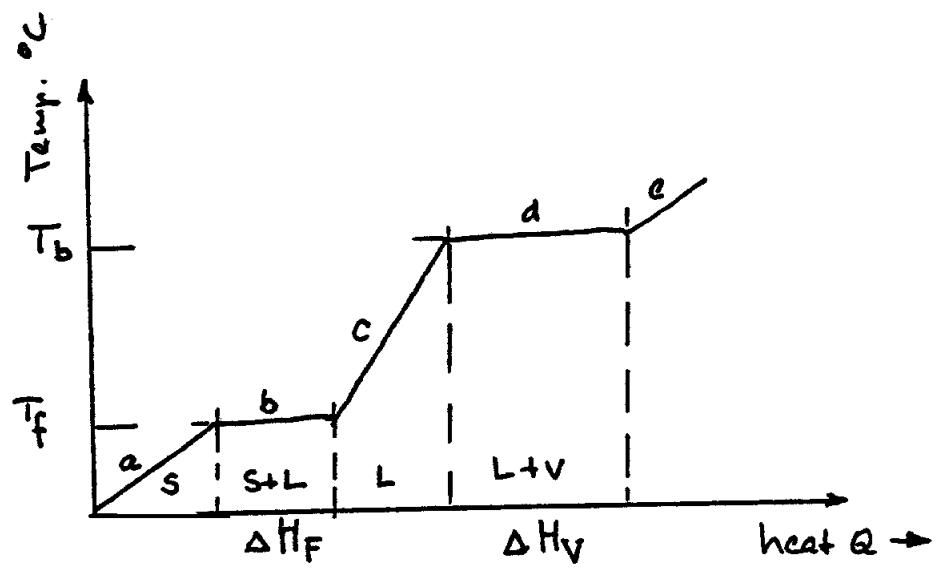
Fig. 2 H vs T Diagram for Pure \(\mathrm{H}_{2} \mathrm{O}\). (Not to scale.)

From a thermodynamic standpoint, it is important to realize that fig. 2 illustrates the energy changes that occur in the system during heating. Actual quantitative measurements show that 5.98 kJ of heat are absorbed at the melting point (latent heat of fusion) and 40.5 kJ per mole (latent heat of evaporation) at the boiling point. The latent heats of fusion and evaporation are unique characteristics of all pure substances. Substances like Fe, Co, Ti and others, which are allotropic (exhibit different structures at different temperatures), also exhibit latent heats of transformation as they change from one solid state crystal modification to another.

ENERGY CHANGES

When heat is added from the surroundings to a material system (as described above), the energy of the system changes. Likewise, if work is done on the surroundings by the material system, its energy changes. The difference in energy \((\Delta \mathrm{E})\) that the system experiences must be the difference between the heat absorbed (Q) by the system and the work (W) done on the surroundings. The energy change may therefore be written as:

\[\Delta \mathrm{E}=\mathrm{Q}-\mathrm{W} \tag{4}\]

If heat is liberated by the system, the sign of \(Q\) is negative and work done is positive. \(Q\) and \(\mathrm{W}\) depend on the direction of change, but \(\Delta \mathrm{E}\) does not. The above relation is one way of representing the First Law of Thermodynamics which states that the energy of a system and its surroundings is always conserved while a change in energy of the system takes place. The energy change, \(\Delta \mathrm{E}\), for a process is independent of the path taken in going from the initial to the final state.

In the laboratory most reactions and phase changes are studied at constant pressure. The work is then done solely by the pressure \((P)\), acting through the volume change, \(\Delta \mathrm{V} .\)

\[\mathrm{W}=\mathrm{P} \Delta \mathrm{V} \quad$ and $\quad \Delta \mathrm{P}=0 \tag{5}\]

Hence:

\[\mathrm{Q}=\Delta \mathrm{E}+\mathrm{P} \Delta \mathrm{V} \tag{6}\]

Since the heat content of a system, or the enthalpy \(\mathrm{H}\), is defined by.

\[\mathrm{H}=\mathrm{E}+\mathrm{PV} \tag{7}\]

\[\Delta \mathrm{H}=\Delta \mathrm{E}+\mathrm{P} \Delta \mathrm{V} \tag{8}\]

so that:

\[\Delta \mathrm{H}=\mathrm{Q}-\mathrm{W}+\mathrm{P} \Delta \mathrm{V} \tag{9}\]

or

\[\Delta \mathrm{H}=\mathrm{Q} \tag{10}\]

Reactions in which \(\Delta \mathrm{H}\) is negative are called exothermic since they liberate heat, whereas endothermic reactions absorb heat. Fusion is an endothermic process, but the reverse reaction, crystallization, is an exothermic one.

ENTROPY AND FREE ENERGY

When a gas condenses to form a liquid and a liquid freezes to form a crystalline solid, the degree of internal order increases. Likewise, atomic vibrations decrease to zero when a perfect crystal is cooled to \(0^{\circ} \mathrm{K}\). Since the term entropy, designated by \(\mathrm{S}\), is considered a measure of the degree of disorder of a system, a perfect crystal at \(0^{\circ} \mathrm{K}\) has zero entropy.

The product of the absolute temperature, \(\mathrm{T}\), and the change in entropy, \(\Delta \mathrm{S}\), is called the entropy factor, T \(\Delta \mathrm{S}\). This product has the same units (Joules/mole) as the change in enthalpy, \(\Delta \mathrm{H}\), of a system. At constant pressure, \(\mathrm{P}\), the two energy changes are related to one another by the Gibbs free energy relation:

\[\Delta \mathrm{F}=\Delta \mathrm{H}-\mathrm{T} \Delta \mathrm{S} \tag{11}\]

where

\[\mathrm{F}=\mathrm{H}-\mathrm{TS} \tag{12}\]

The natural tendency exhibited by all materials systems is to change from one of higher to one of lower free energy. Materials systems also tend to assume a state of greater disorder whereby the entropy factor \(\mathrm{T} \Delta \mathrm{S}\) is increased. The free energy change, \(\Delta \mathrm{F}\), expresses the balance between the two opposing tendencies, the change in heat content \((\Delta \mathrm{H})\) and the change in the entropy factor \((T \Delta S)\).

If a system at constant pressure is in an equilibrium state, such as ice and water at \(0^{\circ} \mathrm{C}\), for example, at atmospheric pressure it cannot reach a lower energy state. At equilibrium in the ice-water system, the opposing tendencies, \(\Delta \mathrm{H}\) and \(\mathrm{T} \Delta \mathrm{S}\), equal one another so that \(\Delta \mathrm{F}=0\). At the fusion temperature, \(\mathrm{T}_{\mathrm{F}}\):

\[\Delta \mathrm{S}_{\mathrm{F}}=\dfrac{\Delta \mathrm{H}_{\mathrm{F}}}{\mathrm{T}_{\mathrm{F}}} \tag{13}\]

Similarly, at the boiling point:

\[\Delta S_v=\frac{\Delta H_v}{T_v} \tag{14}\]

Thus melting or evaporation only proceed if energy is supplied to the system from the surroundings.

The entropy of a pure substance at constant pressure increases with temperature according to the expression:

\[\Delta S=\dfrac{C_p \Delta T}{T} \quad \text { (since }: \Delta H=C_p \Delta T \text { ) } \tag{15}\]

where \(\mathrm{C}_{\mathrm{p}}\) is the heat capacity at constant pressure, \(\Delta \mathrm{C}_{\mathrm{p}}, \Delta \mathrm{H}, \mathrm{T}\) and \(\Delta \mathrm{T}\) are all measurable quantities from which \(\Delta \mathrm{S}\) and \(\Delta \mathrm{F}\) can be calculated.

\(\mathbf{F} \quad \mathbf{v s} \quad \mathbf{T}\)

Any system can change spontaneously if the accompanying free energy change is negative. This may be shown graphically by making use of \(F\) vs \(T\) curves such as those shown in fig. 3.

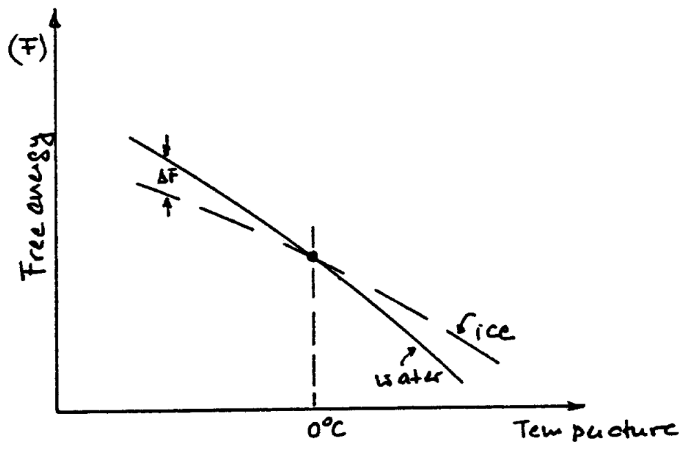
Fig. 3 Free energy is a function of temperature for ice and water.

The general decrease in free energy of all the phases with increasing temperature is the result of the increasing dominance of the temperature-entropy term. The increasingly negative slope for phases which are stable at increasingly higher temperatures is the result of the greater entropy of these phases.

PHASE DIAGRAMS (TWO-COMPONENT SYSTEMS)

SOLID SolutionS

A solution can be defined as a homogeneous mixture in which the atoms or molecules of one substance are dispersed at random into another substance. If this definition is applied to solids, we have a solid solution. The term “solid solution” is used just as “liquid solution” is used because the solute and solvent atoms (applying the term solvent to the element in excess) are arranged at random. The properties and composition of a solid solution are, however, uniform as long as it is not examined at the atomic or molecular level.

Solid solutions in alloy systems may be of two kinds: substitutional and interstitial. A substitutional solid solution results when the solute atoms take up the positions of the solvent metal in the crystal lattice. Solid solubility is governed by the comparative size of the atoms of the two elements, their structure and the difference in electronegativity. If the atomic radii of a solvent and solute differ by more than 15% of the radius of the solvent, the range of solubility is very small. When the atomic radii of two elements are equal or differ by less than 15% in size and when they have the same number of valency electrons, substitution of one kind of atom for another may occur with no distortion or negligible distortion of the crystal lattice, resulting in a series of homogeneous solid solutions. For an unlimited solubility in the solid state, the radii of the two elements must not differ by more than 8% and both the solute and the solvent elements must have the same crystal structure.

In addition to the atomic size factor, the solid solution is also greatly affected by the electronegativity of elements and by the relative valency factor. The greater the difference between electronegativities, the greater is the tendency to form compounds and the smaller is the solid solubility. Regarding valency effect, a metal of lower valency is more likely to dissolve a metal of higher valency. Solubility usually increases with increasing temperature and decreases with decreasing temperature. This causes precipitation within a homogeneous solid solution phase, resulting in hardening effect of an alloy. When ionic solids are considered, the valency of ions is a very important factor.

CONSTRUCTION OF EQUILIBRIUM PHASE DIAGRAMS OF TWO-COMPONENT SYSTEMS

To construct an equilibrium phase diagram of a binary system, it is a necessary and sufficient condition that the boundaries of one-phase regions be known. In other words, the equilibrium diagram is a plot of solubility relations between components of the system. It shows the number and composition of phases present in any system under equilibrium conditions at any given temperature. Construction of the diagram is often based on solubility limits determined by thermal analysis – i.e., using cooling curves. Changes in volume, electrical conductivity, crystal structure and dimensions can also be used in constructing phase diagrams.

The solubility of two-component (or binary) systems can range from essential insolubility to complete solubility in both liquid and solid states, as mentioned above. Water and oil, for example, are substantially insoluble in each other while water and alcohol are completely intersoluble. Let us visualize an experiment on the water-ether system in which a series of mixtures of water and ether in various proportions is placed in test tubes. After shaking the test tubes vigorously and allowing the mixtures to settle, we find present in them only one phase of a few percent of ether in water or water in ether, whereas for fairly large percentages of either one in the other there are two phases. These two phases separate into layers, the upper layer being ether saturated with water and the lower layers being water saturated with ether. After sufficiently increasing the temperature, we find, regardless of the proportions of ether and water, that the two phases become one. If we plot solubility limit with temperature as ordinate and composition as abscissa, we have an isobaric [constant pressure (atmospheric in this case)] phase diagram, as shown in fig. 4. This system exhibits a solubility gap.

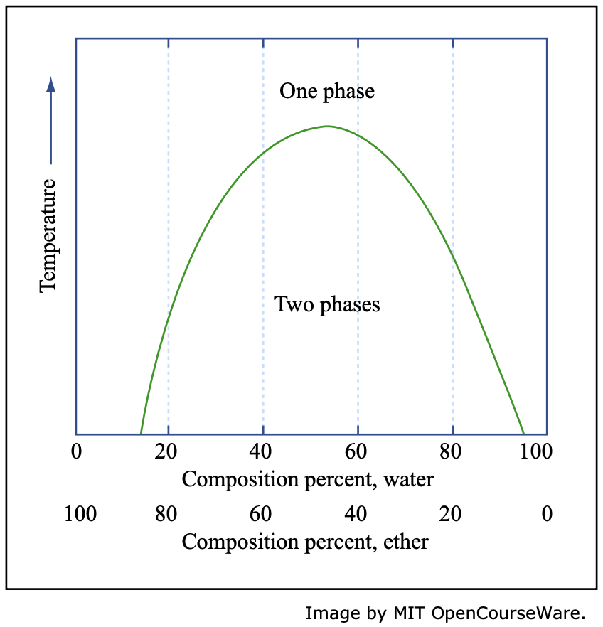
Fig. 4 Schematic representation of the solubilities of ether and water in each other.

COOLING CURVES

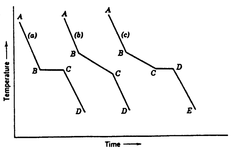
Fig. 5 Cooling curves: (a) pure compound; (b) binary solid solution; (c) binary eutectic system.

SOLID Solution EQUILIBRIUM DIAGRAMS

Read in Jastrzebski: First two paragraphs and Figure 3-4 in Chapter 3-8, "Solid Solutions Equilibrium Diagrams," pp. 91-92.

Read in Smith, C. O. The Science of Engineering Materials. 3rd ed. Englewood Cliffs, NJ: Prentice-Hall, 1986. ISBN: 9780137948840. Last two paragraphs and Figure 7-8 in Chapter 7-3-1, "Construction of a Simple Equilibrium Diagram," pp. 247-248.

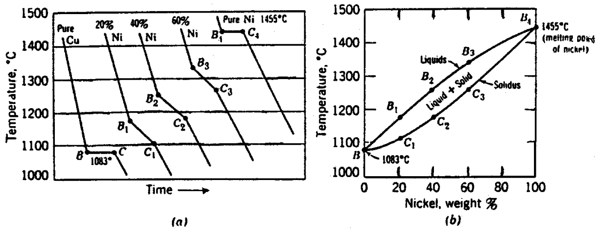
Fig. 6 Plotting equilibrium diagrams from cooling curves for Cu-Ni solid solution alloys. (a) Cooling curves; (b) equilibrium diagram.

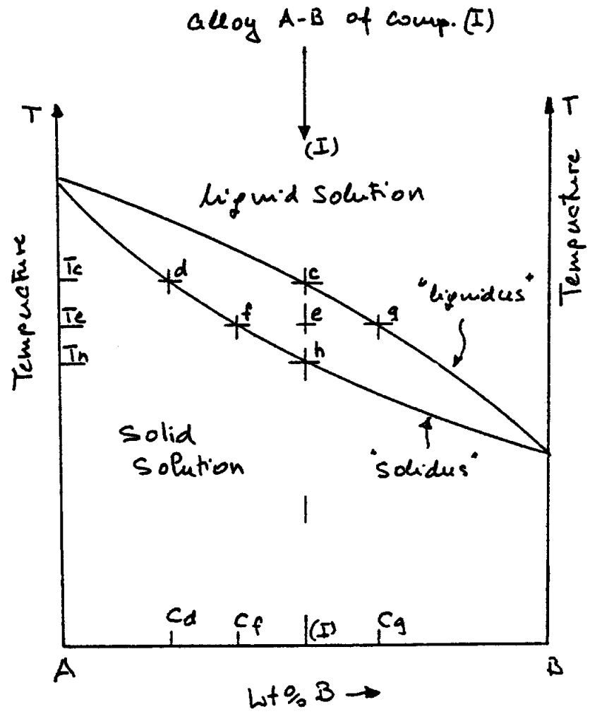
Fig. 7

INTERPRETATION OF PHASE DIAGRAMS

From the above discussion we can draw two useful conclusions which are the only rules necessary for interpreting equilibrium diagrams of binary systems.

Rule 1 - Phase composition: To determine the composition of phases which are stable at a given temperature we draw a horizontal line at the given temperature. The projections (upon the abscissa) of the intersections of the isothermal line with the liquidus and the solidus give the compositions of the liquid and solid, respectively, which coexist in equilibrium at that temperature. For example, draw a horizontal temperature line through temperature \(T_e\) in fig. 7. The \(T_e\) line intersects the solidus at \(f\) and the liquidus at \(g\), indicating solid composition of \(f \%\) of \(B\) and \((100-f) \%\) of \(A\). The liquid composition at this temperature is \(\mathrm{g} \%\) of \(\mathrm{B}\) and \((100-\mathrm{g}) \%\) of \(\mathrm{A}\). This line in a two-phase region is known as a tie line because it connects or "ties" together lines of one-fold saturation - i.e., the solid is saturated with respect to \(B\) and the liquid is saturated with respect to \(A\).

Rule 2 - The Lever Rule: To determine the relative amounts of the two phases, erect an ordinate at a point on the composition scale which gives the total or overall composition of the alloy. The intersection of this composition vertical and a given isothermal line is the fulcrum of a simple lever system. The relative lengths of the lever arms multiplied by the amounts of the phase present must balance. As an illustration, consider alloy I in fig. 7. The composition vertical is erected at alloy I with a composition of \(e \%\) of \(B\) and \((100-e)\%\) of \(A\). This composition vertical intersects the temperature horizontal \(\left(T_e\right)\) at point \(e\). The length of the line " \(f-e-g\) " indicates the total amount of the two phases present. The length of line "\(e-g\)" indicates the amount of solid. In other words:

\begin{aligned}
&\dfrac{\mathrm{eg}}{\mathrm{fg}} \times 100=\% \text { of solid present } \\
&\dfrac{\mathrm{fg}}{\mathrm{fg}} \times 100=\% \text { of liquid present }
\end{aligned}

These two rules give both the composition and the relative quantity of each phase present in a two-phase region in any binary system in equilibrium regardless of physical form of the two phases. The two rules apply only to two-phase regions.

ISOMORPHOUS SYSTEMS

An isomorphous system is one in which there is complete intersolubility between the two components in the vapor, liquid and solid phases, as shown in fig. 9. The \(\mathrm{Cu}-\mathrm{Ni}\) system is both a classical and a practical example since the monels, which enjoy extensive commercial use, are \(\mathrm{Cu}-\mathrm{Ni}\) alloys. Many practical materials systems are isomorphous.

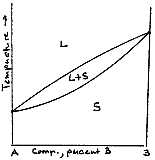
Fig. 9 Schematic phase diagram for a binary system, A-B, showing complete intersolubility (isomorphism) in all phases.

INCOMPLETE SOLUBILITY

Read in Smith, C. O. The Science of Engineering Materials. 3rd ed. Englewood

Cliffs, NJ: Prentice-Hall, 1986. ISBN: 9780137948840.

Chapter 7-3-5, "Incomplete Solubility," pp. 252-253.

EUTECTIC SYSTEMS

Read in Smith: Chapter 7-3-6, "Eutectic," pp. 253-256.

EQUILIBRIUM DIAGRAMS WITH INTERMEDIATE COMPOUNDS

Read in Jastrzebski, Z. D. The Nature and Properties of Engineering Materials. 2nd ed.

New York, NY: John Wiley & Sons, 1976. ISBN: 9780471440895.

Chapter 3-11,"Equilibrium Diagrams with Intermediate Compounds," pp. 102-103.

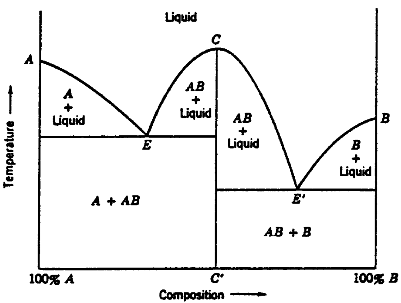
Fig. 15 Binary system showing an intermediate compound. C is the melting point (maximum) of the compound AB having the composition C’. E is the eutectic of solid A and solid AB. E’ is the eutectic of solid AB and solid B.

 

TWO-COMPONENT SYSTEMS

A pressure-temperature diagram is extremely useful when one wishes to discuss a one-component system. A component in this case is an element or compound (for example, Fe, MgO, or \(\mathrm{H}_{2} \mathrm{O}\)). As long as there is only one component present, the system may be adequately described by the two variables, pressure and temperature. In a two-component system, a third variable is needed; this is composition. The two-component system may be described by a three dimensional pressure - temperature composition diagram. It is however in the framework of this course not appropriate to deal with the complexities of the 3D phase diagram at this point and, since most materials are used under isobaric (constant pressure) conditions, we will first discuss an isobaric two-dimensional diagram of temperature versus composition. At a later point we will explain how the one component pressure-temperature and the isobaric two-component temperature-composition diagrams may be combined to construct the three-dimensional pressure-temperature-composition diagram of a two-component system.

Temperature-composition diagrams

A two-component temperature-composition diagram at constant pressure is called a binary phase diagram or equilibrium diagram. Temperature is plotted as the ordinate and composition as the abscissa. In the system \(A B\), the composition is usually expressed in terms of the mole fraction of \(B, x_B\), or the weight percent of \(B\), w/o \(B\). (The mole fraction of \(B\) is equal to the number of moles of \(B\) divided by the sum of the number of moles of \(A\) plus the number of moles of \(B\). The weight percent of \(B\) is equal to the product of 100 and the weight of \(B\) divided by the sum of the weights of \(A\) and \(B\).) The composition need not be specified in terms of \(A\) since the sum of the mole fraction of \(B\) and the mole fraction of \(A\) is equal to one, and the sum of the weight percent of \(A\) and the weight percent of \(B\) is equal to 100. For pure \(A\), both \(x_B\) and w/o \(B\) are zero; and for pure \(B\) they are one and 100, respectively.

A typical binary phase diagram (Figure 1) indicates those phases present in equilibrium at any particular temperature and composition at the constant pressure for which the phase diagram was determined. At low temperatures, the only phase present is the solid designated by \(S\) in the phase diagram. Pure \(A\) melts at the temperature \(T_{f A}\) and pure \(B\) melts at the temperature \(T_{fB}\) Alloys of composition between pure \(A\left(x_B=0\right)\) and pure \(B\left(x_B=1\right)\) exist only in the solid state of aggregation until the temperature of the solidus line is reached. The solidus is represented in the phase diagram by the lower curve extending from \(\mathrm{T}_{\mathrm{fA}}\) to \(\mathrm{T}_{\mathrm{fB}}\). Below the solidus temperature only solid exists; but above the solidus, there is a two-phase region \((L+S)\) in which both liquid and solid phases are in equilibrium. The liquid-plus-solid region extends from the solidus temperature over a finite temperature interval for all alloys of the system \(A B\). The extent of the temperature interval reduces to zero for the pure components \(A\) and \(B\). since according to the one-component pressure-temperature diagram, at any particular pressure there is only one temperature at which liquid and solid are in equilibrium.

Figure 1 • Binary Phase Diagram. A binary phase diagram is an isobaric temperature composition diagram. In this case there is complete volubility in the solid, liquid, and vapor states of aggregation, and only one phase is found for each state of aggregation. At low temperatures, the material of any composition is solid; at higher temperatures there is a two-phase liquid-plus-solid region, a liquid region, a liquid-plus-vapor region and, at very high temperatures, an all-vapor region.

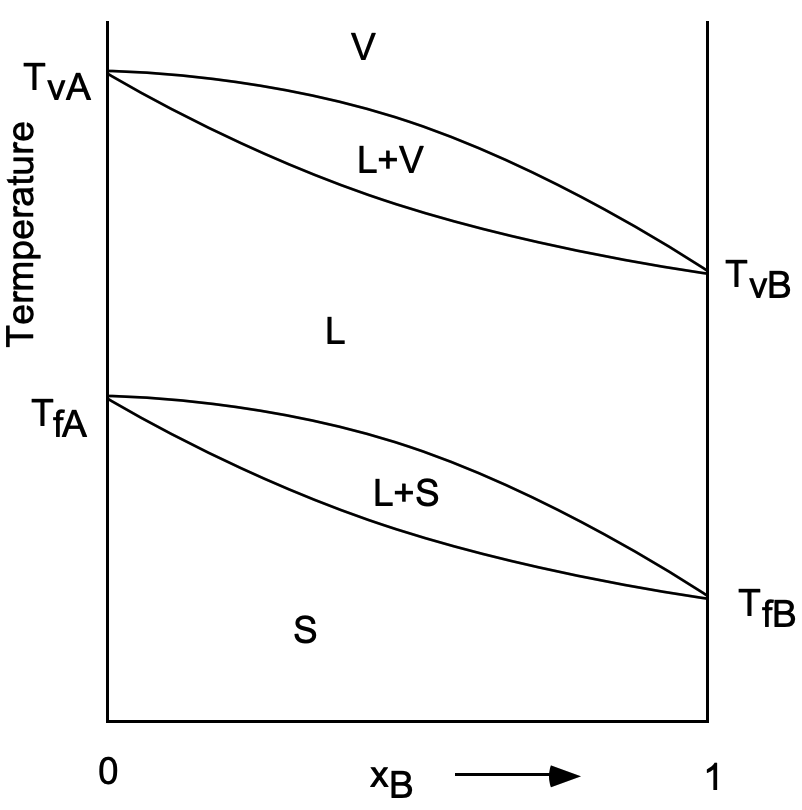
The upper boundary of the liquid-plus-solid region is the liquidus temperature. Above this temperature, any alloy of the system exists as a liquid phase until the temperature increases to that level at which vaporization begins. The pure compositions A and B vaporize completely at \(T_{v A}\) and \(T_{v B}\), because the liquid and vapor phases for a pure component at constant pressure can be in equilibrium at only one temperature. Alloys of intermediate composition do not completely vaporize at any one temperature but over a finite temperature interval.This is shown in the phase diagram of Figure 1 by the liquid-plus-vapor \((L+V)\) region. At temperatures above this region, only the vapor phase exists.

Metallurgists or materials scientists are more often concerned with the liquid and solid phases and less often with the vapor phase. For this reason, and the fact that it is difficult to determine vapor phase diagrams, most binary diagrams extend no higher in temperature than the all-liquid region.

Cooling through a two-phase field

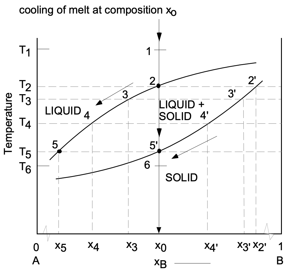
Solidification or melting of an intermediate alloy may be illustrated by the enlarged view of a two-phase field shown in Figure 2.

If an alloy of composition \(\mathrm{x}_{\mathrm{o}}\), originally liquid at temperature \(\mathrm{T}_1\), is cooled, it remains liquid until the temperature reaches the liquidus temperature at point 2. At this temperature \(T_2\), the first particle of solid appears. This solid does not have the same composition as the parent liquid. The composition of the first solid formed at \(\mathrm{T}_2\) is found by constructing an isothermal line from 2 to \(2^{\prime}\). This isotherm is called a tie-line. The composition of the solid and liquid phases in equilibrium at a particular temperature is given by the intersection of the tie-line at that temperature with the solidus and liquidus curves, respectively. Thus at temperature \(T_2\), the solid has the composition \(\times 2^{\prime}\) and the liquid the composition \(x_2\) (where \(x_2=x_0\) ).

Upon further cooling to \(T_3\), the composition of the liquid has shifted to the left along the liquidus to \(\times 3\), and the composition of the solid has shifted to the left along the solidus to \(x 3^{\prime}\) because at \(T_3\), the only liquid and solid compositions that can be in equilibrium with one another are \(x 3\) and \(x 3^{\prime}\) respectively.

Despite the fact that both liquid and solid have compositions different from the alloy composition, the overall alloy (liquid and solid together) retains its original composition \(x_0\). As the temperature approaches the solidus temperature \(\mathrm{T}_5\), the solid composition approaches \(x^{\prime}\), (where \(x_5{ }^{\prime}=x_0\) ) and the last quantity of liquid of composition \(x_5\) freezes. At temperatures below the solidus, the solid composition remains unchanged, for example, at \(\mathrm{T}_6\) the solid composition is \(\mathrm{x}_0\).

The above analysis applies only to solidification at such a slow rate of cooling that equilibrium is achieved at every temperature. This is not always the case, however.

Figure 2 \(\cdot\) Cooling Through a Two-Phase Field. As an alloy of composition \(x_0\) is cooled from the liquid region through the two-phase liquid-plus-solid field, the first particle of solid forms at temperature \(T_2\) and is of composition \(x_2\),. The composition of the solid is given by the intersection of the isothermal tie line with the solidus, and the composition of the liquid by the intersection of the tie-line with the liquidus. As the temperature is decreased, the composition of the solid and of the liquid shifts to the left until at \(\mathrm{T}_5\) the solid is of composition \(\mathrm{x}_0\) and the last of the liquid freezes.

lever law

To determine exactly how much liquid and solid are present at any given temperature, let us derive a relation known as the "lever law." If one mole of alloy of composition \(x_0\) is chosen as a basis, then, at any temperature \(T\). the fraction of liquid \(f_L\) is found as follows: The sum of the fractions of liquid and solid must equal one, that is,

\(f_S+f_L=1\)

The number of moles of B present in the alloy must be the same as the number of moles of B present in the solid phase plus the number of moles of B present in the liquid phase, that is,

\(x_O=x_S f_S=x L f_L\)

Since

\(f_S=1-f_L\)

we may substitute and obtain

\(x_O=x_S-x_S f L+x_L f_L\)

On rearranging and solving for \(\mathrm{f}_\mathrm{L}\) we find that

\(f_L=\left(x_S-x_0\right) /\left(x_S-x L\right) .\)

This relation is called the "lever law" because the fraction of one of the two phases present is equal to the opposite side of the tie-line \(\left(\mathrm{x}_{\mathrm{S}}-\mathrm{x}_{\mathrm{O}}\right)\) divided by the entire tie-line \(\left(x_S-x_L\right)\) In this way the tie-line acts as though it were a lever whose fulcrum is at the point \(x_0\). In a similar way it is found that

\(f_s=\left(x_O-x_L\right) /\left(x_S-x L\right) .\)