1.8: Theory of Reaction Rates

1. INTRODUCTION

We can readily understand that chemical reactions normally are preceded by collisions of atoms, ions, or molecules. However, the rate of such collisions in solids, liquids and gases is so great that all reactions would be very rapid were it only necessary for collisions to occur. “Chemical” reactions will not proceed more rapidly than molecular collisions allow, but many reactions proceed much more slowly. It is thus apparent that not every molecular collision leads to reaction. We have also seen from earlier examples that the driving force for physical as well as chemical reactions is the (free) energy change - which must be negative for reactions to occur spontaneously. However, while providing a “go/no-go” answer, this criterion alone cannot give us any information concerning the rate at which reactions occur, nor can it tell us which factors influence the reaction velocity.

Rates at which reactions occur vary considerably. For example, the nuclear reaction:

\begin{aligned}
&\mathrm{U}_{92}^{238} \rightarrow \mathrm{Th}_{90}^{234}+\alpha \quad &&\text{is } 50 \% \text{ completed } \left(\tau_{1 / 2}\right) \text{ after } 5 \times 10^9 \text{ years}. \\ \\
&\tau_{1 / 2}=5 \times 10^9 \text{years}
\end{aligned}

On the other hand, the chemical reaction:

\begin{aligned}
\mathrm{SO}_4^{-}+\mathrm{H}^{+} &\rightarrow \mathrm{HSO}_4^{-} \quad &&\text{is } 50\% \text{ completed after about } 10^{-4} \mathrm{~s}. \\
\tau_{1 / 2}&=3 \times 10^{-4} \quad &&\text{seconds}
\end{aligned}

Reaction kinetics (rate theory) deals to a large extent with the factors which influence the reaction velocity. Take corrosion (rusting of iron), for example. We all know that it requires air and water to provoke rusting and we also know, much to our sorrow, that rusting proceeds much more rapidly near the ocean where salt is present. We also know that the rate of rusting depends strongly on the composition of iron (pure Fe and steel corrode much less rapidly than cast iron, for example). It is primarily kinetic studies which lead to the elucidation of chemical reactions and, in the case of corrosion, to the development of more corrosion resistant materials.

The principal experimental approach to the study of the reaction process involves the measurement of the rate at which a reaction proceeds and the determination of the dependence of this reaction rate on the concentrations of the reacting species and on the temperature. These factors are grouped together in the term reaction kinetics and the results for a given reaction are formulated in a rate equation which is of the general form:

Rate = k(T) x function of concentration of reactants

The quantity k(T) is called the rate constant and is a function only of the temperature if the term involving the reactant concentrations correctly expresses the rate dependence on concentration. Thus the experimental information on the reaction process is summarized in the rate equation by the nature of the concentration function and by the value and temperature dependence of the rate constant.

2. EXPERIMENTAL METHODS IN REACTION RATE STUDIES

Since we know that chemical reactions are temperature dependent, kinetic investigations will require rigorous temperature control (thermostats). Furthermore, we have to be able to observe and investigate concentration changes of reactions and products. For this purpose it frequently is customary to interrupt a reaction (for example, by quenching - the abrupt lowering of temperature) and to make a chemical analysis. In other instances, particularly for very fast reactions, a direct measurement of concentration changes is physically impossible. In such cases it is necessary to quantitatively follow reactions indirectly, through the accompanying changes in specific physical properties such as:

(1) electrical conductivity

(2) optical absorption

(3) refractive index

(4) volume

(5) dielectric constant

as well as by other means. In the last twenty years, for example, the use of isotopes (as “tracer” elements) has become a valuable tool for the study of reaction kinetics (in slow reactions).

3. CONCENTRATION DEPENDENCE OF REACTION RATES

Normally experimental data of kinetic investigations are records of concentrations of reactants and/or products as a function of time for constant temperatures (taken at various temperatures).

Theoretical expressions for reaction rates (involving concentration changes) are differential equations of the general form:

\(\dfrac{\mathrm{dc}}{\mathrm{dt}}=\mathrm{f}\left(\mathrm{c}_1^{\mathrm{m}}, \mathrm{c}_2^{\mathrm{n}}, \mathrm{c}_3^{\mathrm{o}} \ldots\right)\)

where (c) are concentration terms which have exponents that depend on details of the reaction.

If we want to compare the theory with the experiment, it is therefore necessary to either integrate the theoretical laws or to differentiate experimental concentration vs time data.

The rate laws are of importance since they provide analytical expressions for the course of individual reactions and enable us to calculate expected yields and optimum conditions for “economic” processes.

In most instances the differential rate equation is integrated before it is applied to the experimental data. Only infrequently are slopes of concentration vs time curves taken to determine dc/dt directly (fig. 1).

Figure 1 Variation with time of the concentration of a reactant (A) and of a product (B)

Let us look at a simple reaction, the decay of \(\mathrm{H}_2 \mathrm{O}_2\) to water and oxygen:

\(2 \mathrm{H}_2 \mathrm{O}_2 \rightarrow 2 \mathrm{H}_2 \mathrm{O}+\mathrm{O}_2\)

Figure 2 Decay curve (dc/dt vs. c) for \(\mathrm{H}_2 \mathrm{O}_2\)

Experimentally we obtain a curve (such as fig. 2) by plotting the concentration of remaining \(\mathrm{H}_2 \mathrm{O}_2\) in moles/liter, normally written [\(\mathrm{H}_2 \mathrm{O}_2\)], as a function of time. The rate is then given by the time differential:

Rate \(\left(\dfrac{\text { moles }}{\text { liter } \cdot \mathrm{s}}\right)=\dfrac{-\mathrm{d}\left[\mathrm{H}_2 \mathrm{O}_2\right]}{\mathrm{dt}}\)

If we now determined and plotted the variation of the reaction rate, \(\left[-\mathrm{d}\left[\mathrm{H}_2 \mathrm{O}_2\right] /(\mathrm{d}\right.\) time \(\left.)\right]\), with concentration, \(\left[\mathrm{H}_2 \mathrm{O}_2\right]\), we would find a straight line (fig. 3). Thus:

\(-\dfrac{\mathrm{d}\left[\mathrm{H}_2 \mathrm{O}_2\right]}{\mathrm{dt}}=\mathrm{k}\left[\mathrm{H}_2 \mathrm{O}_2\right]\) or generally, \(-\dfrac{\mathrm{dc}}{\mathrm{dt}}=\mathrm{kc}\)

Upon integration:

\(\int \dfrac{d c}{c}=-k \int d t\)

we have:

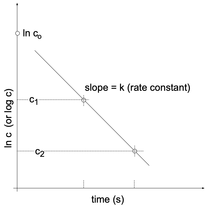
\(\ln  \mathrm{c}=-\mathrm{kt}+\text { const. }\)

Taking \(\mathrm{c}=\mathrm{c}_{\mathrm{o}}\) for \(\mathrm{t}=0\), we get \(\left(\right.\) const \(\left.=\ln \mathrm{c}_{\mathrm{o}}\right)\) and:

\(\ln \mathrm{c}=-\mathrm{kt}+\ln \mathrm{c}_{\mathrm{o}}\)

or:

\(\mathrm{c}=\mathrm{c}_{\mathrm{o}} \mathrm{e}^{-\mathrm{kt}} \quad \text { and } \quad \mathrm{k}=\dfrac{1}{\mathrm{t}} \times \ln \dfrac{\mathrm{c}_{\mathrm{o}}}{\mathrm{c}}\)

Figure 3 Concentration dependance of the rate of reaction

Alternately:

\(k=\dfrac{2.3}{t} \times \log \dfrac{c_0}{c} \quad \text { and } \quad k=\dfrac{2.3}{t_2-t_1} \times \log \dfrac{c_1}{c_2}\)

From the above we see that for decay of \(\mathrm{H}_2 \mathrm{O}_2\) a plot of \((\ln \mathrm{c})\) vs. \(t\) results in a straight line (fig. 4). This behavior is characteristic of first order reactions in which the concentration exponent \((\mathrm{n})\) is "one":

\(-\dfrac{\mathrm{dc}}{\mathrm{dt}}=\mathrm{kc}\)

First Order Reactions: Radioactive Decay

From the relationship:

\(\mathrm{k}=\dfrac{2.3}{\mathrm{t}_2-\mathrm{t}_1} \times \log \dfrac{\mathrm{c}_1}{\mathrm{c}_2}\)

which relates the rate constant \((k)\) to the concentration change \((\Delta c)\) for the time interval \((\Delta t)\), we can show that (for first order reactions) the time required to complete a reaction to \(1 / 2\) or \(1 / 4\) or any fraction of the initial concentration is independent of the initial concentration of reactant present (fig. 5).

Figure 4 Plot of ln c vs. time

 

Figure 5 Concentration independent half life (t.5) of First order reactions.

When discussing radioactive decay it is customary to call the “rate constant” (k) the “decay constant”. It is furthermore customary to consider the time it takes to decrease the number of originally present species (normally called reactants) to 0.5 (by 50%). We then talk about the half-life. Accordingly, the above equation can be reformulated as:

\(\mathrm{k}=\dfrac{2.3}{\mathrm{t}_{1 / 2}} \times \log \dfrac{\mathrm{c}_1}{\dfrac{\mathrm{c}_1}{2}}=\dfrac{2.3}{\mathrm{t}_{1 / 2}} \times \log 2\)

or:

\(k=\dfrac{0.693}{t_{1 / 2}}\)

This means that from the half-life \(\left(\mathrm{t}_{1 / 2}\right)\) we may obtain the decay constant (rate constant in general). Vice versa, knowing the rate constant, we can calculate the time it takes to complete \(50 \%\) of the reaction (or decay).

4. REACTION ORDER

Reactions of first order, such as the decay of \(\mathrm{H}_2 \mathrm{O}_2\) or radioactive decay, do not require molecular or atomic collisions - in principle they reflect inherent instability. A multitude of chemical reactions do involve collisions, however. For example, take the decay of HI:

\(2 \mathrm{HI} \rightarrow \mathrm{H}_2+\mathrm{I}_2\)

The rate law for this reaction reflects the requirement of a collision in the concentration exponent:

\(-\dfrac{\mathrm{d}[\mathrm{HI}]}{\mathrm{dt}}=\mathrm{k}[\mathrm{HI}] \times[\mathrm{HI}]=k[H \mathrm{H}]^2\)

The reaction is referred to as a second order reaction which can readily be identified since upon integration the rate law yields:

\(\dfrac{1}{[\mathrm{HI}]}=\mathrm{kt}+\text { const }\)

or, more generally:

\(\dfrac{1}{\mathrm{c}}=\mathrm{kt}+\text { const }\)

A plot of \(1 / c\) vs \(t\) will yield a straight line.

It is interesting to note that a determination of the reaction order from experimental data supplies insight to the details of how molecules and atoms react with each other. Even though rate data involve measurements of gross numbers of molecules, their interpretation (through the reaction order) permits us to formulate the probable step (or steps) which individual molecules undergo.

5. TEMPERATURE DEPENDENCE OF REACTION RATES

Although a chemical reaction may be "thermodynamically" favored (which means the free energy of the system will be lowered as a result of the reaction), reaction may nevertheless not take place. Thus, \(\mathrm{H}_2\) and \(\mathrm{O}_2\) gases can exist in intimate contact over a considerable temperature range before reaction takes place. Nevertheless, a lighted match or a platinum powder catalyst can nucleate an immediate explosive reaction. Another example with which we are familiar is glass: some glasses remain "supercooled liquids" for thousands of years at room temperature unless reheated to some definite temperature for at least some minimum period of time. Many different factors may influence the rate of a reaction - for example:

(1) Existing interatomic (or intermolecular) bonds must be broken.

(2) Atoms must be moved to and away from the reaction site.

(3) A new boundary is required wherever a new "phase" is to be nucleated.

All three steps cited require work or a supply of energy. Furthermore, all three steps are temperature dependent. At the beginning of this chapter we have stated:

Rate \(=k(T) \times\) function of concentration of reactants

In other words: the reaction rate is proportional to the concentration of reactants. The proportionality constant \(k\) is a function of temperature \(k(T)\). The temperature dependence of \(k\) (which represents the temperature dependence of the rate of a given reaction) can be studied by performing experiments (with constant concentrations) at different temperatures. From such experiments it can be seen that the value of the rate constant (\(k\)) is much greater at higher temperatures - the reactions proceed faster

In 1899 Arrhenius showed that the rate constant of reactions increased in an exponential manner with T. By an empirical procedure he found that a plot of log k versus 1/T gives a linear relation.

Remember: In all kinetic and thermodynamic calculations it is mandatory to use the "absolute temperature scale" in Kelvin (K) which is given by:

\(\mathrm{K}={ }^{\circ} \mathrm{C}+273.16\)

Thus OK \(=-273.16 \mathrm{C}\), which corresponds to the thermodynamic absolute zero temperature. Linear plots of \(\log \mathrm{k}\) vs \(1 / \mathrm{T}\) imply the relation:

\(\ln k \propto \dfrac{1}{T}\)

\(k \propto e^{\text {const/T }}\)

In view of later deductions this empirical relation can be conveniently written as:

\(\mathrm{k}=\mathrm{A} \mathrm{e}^{-\mathrm{E} / \mathrm{RT}}\)

where \(A\) is a proportionality constant sometimes called the reaction constant, \(R\) is the gas constant and equals \(8.31 \mathrm{~J} /\) mole \(\mathrm{K}, \mathrm{E}\) is the activation energy in Joules/mole and e is the base of the natural (Naperian) system of logarithms. Since \(\ln x=2.3 \log _{10} x\), we can rewrite the above equation:

\(\ln \mathrm{k}=\ln \mathrm{A}-\dfrac{\mathrm{E}}{\mathrm{RT}}\)

or

\(\log k=\log A-\dfrac{E}{2.3 \times 8.3 \times \mathrm{T}}\)

Figure 6 Arrhenius plot permitting the determination of activation energies

If the above equation is obeyed, a plot of log k versus 1/T (fig. 6) will be a straight line from which the characteristic activation energy can be determined since the slope is –E/19.15. The reaction constant (log A) may in turn be evaluated by extrapolating the rate line to the point at which 1/T equals zero.

It is important to realize that many reactions involve a succession of steps, in which case the rate is controlled by the slowest step. The corresponding values of E and A must be determined by experimental methods.

6. THE ARRHENIUS THEORY

Arrhenius developed a primarily qualitative theory for molecular reactions which led to empirical expressions for the rate constant. Later theories (which are beyond the scope of 3.091) elaborate and make these original ideas more quantitative.

The very simple (reversible) vapor-phase reaction of hydrogen and iodine to give hydrogen iodide can be used to illustrate the ideas of Arrhenius. The reaction

\(\mathrm{H}_2+\mathrm{I}_2 \rightarrow 2 \mathrm{HI}\)

apparently proceeds by a one-step (one collision) four-center process such that the path of the reaction can be depicted as follows:

For more complicated systems, even when a mechanism has been postulated, it is not so easy to see how the electrons and atoms move around as the reaction proceeds. However, even Arrhenius recognized that any reaction process can proceed first by means of the formation of some “high-energy species” (which we now call the “activated-complex”) and secondly by the breakdown of this complex into products.

If the activated-complex is assumed to have an energy, \(\mathrm{E}_{\mathrm{a}}\), greater than the reactants, then, in analogy to earlier considerations, the number of activated-complex molecules compared with the number of reactant molecules can be written in terms of the Boltzmann distribution as:

\(\dfrac{\text { [activated }-\text { complex molecules] }}{[\text { reactant] }}=e^{-E_a / R T}\)

The rate of reaction thus becomes proportional to the concentration of activated-complex molecules:

\(\text{Rate} \propto (\text{activated-complex molecules})\)

or

\(\text { Rate }=A \times e^{-E_a / R T} \times \text { reactants }\)

Making

\(k=A e^{-E_a / R T}\)

we find

\(\text { Rate }=\mathrm{k} \text { [reactants] }\)

Moreover, the theory says that the empirical constant, \(\mathrm{E}_{\mathrm{a}}\), is to be interpreted as the energy of the activated-complex compared with that of the reactant molecules.

The idea of an activated-complex can be presented on a plot (fig. 7) of the energy of

Figure 7 Schematic of a reaction via activated complex formation

the system as ordinate versus the reaction coordinate as abscissa. The reaction coordinate is not any single internuclear distance, but rather depends on all the internuclear distances that change as the reactant molecules are converted into product molecules. In general it is impossible, and for the present purpose unnecessary, to give a quantitative description of the reaction coordinate. It consists of the transformation from reactants to products.

The Arrhenius theory leads to a considerable improvement in our understanding of the reaction process. It is, however, still a very qualitative theory in that it does not show how the pre-exponential factor A depends on the molecular properties of the reaction system, nor does it attempt to predict the value of \(\mathrm{E}_{\mathrm{a}}\).

7. THE ACTIVATION ENERGY

The basic distribution of molecular (or atomic) energies at two different temperatures is given in fig. 8. It can be shown that \(e^{-E_a / R T}\) is the fraction of molecules or atoms having

Figure 8 Maxwell Boltzmann energy distribution

an energy of \(\mathrm{E}_{\mathrm{a}}\) or greater. The Arrhenius equation holds only if the interacting species have between them at least the certain critical energy \(\mathrm{E}_{\mathrm{a}}\). Since the fraction having this energy or greater is \(e^{-E_a / R T}\), the reaction rate is proportional to this quantity.

As the value of \(\mathrm{E}_{\mathrm{a}}\) increases, the energy requirement increases and it becomes more difficult for the molecules to acquire this energy. In contrast, \(e^{-E_a / R T}\) increases rapidly with increasing temperature (T).

The change of a reaction rate with increasing temperature is usually much greater than expected from the corresponding increase in the average velocity of molecules and atoms. The average velocity of molecules and atoms is proportional to the square root of the absolute temperature. Thus, if the temperature is raised \(10^{\circ}\) from \(298^{\circ}\) to \(308^{\circ}\), the average velocity increase, \((308 / 298)^{1 / 2}\), is but \(2 \%\) whereas the rate of reaction increases by about \(100 \%\). From this we must conclude that the reaction rate is controlled not only by the number of collisions, but also by the activation energy.

We now realize that in order for a reaction to proceed we have to supply activation energy. We also know that for given conditions of concentration and T the rate of any reaction is inversely proportional to the energy of activation.

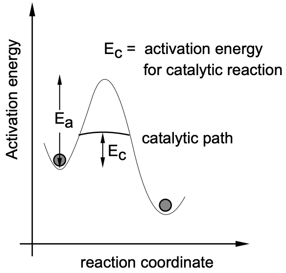
Since, particularly in industry, time is a major factor which can make a process economically feasible or unfeasible, considerable efforts have been put into accelerating reactions by means of catalysts. In catalytic reactions the “catalyst”, which effectively lowers the required activation energy (fig. 9), is characterized by the following criteria:

(1) unchanged chemically at the end of a reaction;

(2) required in small amounts only;

(3) catalytic action is frequently proportional to its surface area;

(4) catalysis can be selective: if different reactions are possible, catalysis can enhance the rate of either one without affecting the alternate reaction.

Figure 9 Effect of catalysis on activation energy in chemical reaction.

For example:
\begin{aligned}
\mathrm{C}_2 \mathrm{H}_5 \mathrm{OH} \rightarrow & \mathrm{H}_2 \mathrm{C}=\mathrm{CH}_2+\mathrm{H}_2 \mathrm{O} & \text { on } \gamma \text { Alumina } \\
& \text { (important in polymer chemistry) } \\
&\left(\gamma \text { Alumina: a cubic form of } \mathrm{Al}_2 \mathrm{O}_3\right) \\
\mathrm{C}_2 \mathrm{H}_5 \mathrm{OH} \rightarrow & \mathrm{CH}_3-\mathrm{C}_H^{\prime \mathrm{O}}+\mathrm{H}_2 \quad &\text { on Copper }
\end{aligned}

While the exact action of catalysis is still quite unclear, we do have some concrete information. The most frequently encountered case, heterogeneous catalysis (the presence of certain solids which increase gas reactions) is attributed to activation by adsorption. From infrared studies we know that upon adsorption of compounds the bonds within the compound are weakened and reactions can subsequently occur with decreased activation energy.

Catalysis has certainly had considerable impact on our daily life. Until 1940 gasoline was exclusively made from crude oil. Also, possibly more important, nitrates and ammonia came primarily from Chile (Chile saltpeter). In the Fischer-Tropsch process, coal and steam are converted into gasoline hydrocarbons with the aid of \(\mathrm{Ni}-\mathrm{Co}\) catalysts. The Haber-Bosch process, \(\mathrm{N}_2+3 \mathrm{H}_2 \rightarrow 2 \mathrm{NH}_3\) (ammonia) \(+99 \mathrm{~kJ}\), is likely the most important catalytic reaction practiced: From the "Le Chatelier" principle (if in a reaction the number of molecules present decreases, the reaction can be accelerated by applying increased pressures) we know that high pressures will favor this synthesis, but we also know that high temperature will favor the reverse reaction, i.e., decay of ammonia; at high temperatures complex molecular structures tend to decay to more elemental, basic species. Catalysis \(\left(\mathrm{Fe}, \mathrm{Al}_2 \mathrm{O}_3+\mathrm{K}_2 \mathrm{O}\right.\) in solid form) makes it possible at \(400^{\circ} \mathrm{C}\) and at about 600 atm to convert about \(60 \%\) of the gas mixture \(\mathrm{N}_2+3 \mathrm{H}_2\) to \(\mathrm{NH}_3\). Nitrates (important as fertilizers and explosives) are predominantly produced by catalytic oxidation.

\begin{aligned}
&4 \mathrm{NH}_3+5 \mathrm{O}_2 \rightarrow 4 \mathrm{NO}+6 \mathrm{H}_2 \mathrm{O} \quad \text { over Pt at } 900^{\circ} \mathrm{C} \\
&2 \mathrm{NO}+\mathrm{O}_2 \rightarrow 2 \mathrm{NO}_2 \\
&3 \mathrm{NO}_2+\mathrm{H}_2 \mathrm{O} \rightarrow 2 \mathrm{HNO}_3 \text { (nitric acid) }+\mathrm{NO}
\end{aligned}

Other examples are:

* \(\mathrm{SO}_2+1 / 2 \mathrm{O}_2 \rightarrow \mathrm{SO}_3\) over \(\mathrm{V}_2 \mathrm{O}_5\)

* Synthetic rubber from butadiene and styrene

* Methanol from \(\mathrm{CO}+2 \mathrm{H}_2 \rightarrow \mathrm{CH}_3 \mathrm{OH}\) over \(\mathrm{ZnO}+\mathrm{Cr}_2 \mathrm{O}_3\)

* Formaldehyde from  over \(\mathrm{Cu}\) (important for plastics)

* In nature we have a large number of catalysts in the form of enzymes.