8.5: Equilibrium

Now that we have a good idea about the factors that affect how fast a reaction goes, let us return to a discussion of what factors affect how far a reaction goes. As previously discussed, a reaction reaches equilibrium when the rate of the forward reaction equals the rate of the reverse reaction, so the concentrations of reactants and products do not change over time. The equilibrium state of a particular reaction is characterized by what is known as the equilibrium constant, \(\mathrm{K}_{eq}\).

We can generalize this relationship for a general reaction: \[n\mathrm{A}+m\mathrm{B} \rightleftarrows o\mathrm{C}+p\mathrm{D} .\]

Note that each concentration is raised to the power of its coefficient in the balanced reaction. By convention, the constant is always written with the products on the numerator, and the reactants in the denominator. So large values of \(\mathrm{K}_{eq}\) indicate that, at equilibrium, the reaction mixture has more products than reactants. Conversely, a small value of \(\mathrm{K}_{eq}\) (typically <1, depending on the form of \(\mathrm{K}_{eq}\)) indicates that there are fewer products than reactants in the mixture at equilibrium. The expression for \(\mathrm{K}_{eq}\) depends on how you write the direction of the reaction. You can work out for yourself that \(\mathrm{K}_{eq} (\text{forward})= 1/\mathrm{K}_{eq}(\text{reverse})\). One other thing to note is that if a pure liquid or solid participates in the reaction, it is omitted from the equilibrium expression for \(\mathrm{K}_{eq}\). This makes sense because the concentration of a pure solid or liquid is constant (at constant temperature). The equilibrium constant for any reaction at a particular temperature is a constant. This means that you can add reactants or products and the constant does not change.^[16] You cannot , however, change the temperature, because that will change the equilibrium constant as we will see shortly. The implications of this are quite profound. For example, if you add or take away products or reactants from a reaction, the amounts of reactants or products will change so that the reaction reaches equilibrium again—with the same value of \(\mathrm{K}_{eq}\). And because we know (or can look up and calculate) what the equilibrium constant is, we are able to figure out exactly what the system will do to reassert the equilibrium condition.

Let us return to the reaction of acetic acid and water: \[\mathrm{ACOH}+\mathrm{H}_{2} \mathrm{O} \rightleftarrows \mathrm{H}_{3} \mathrm{O}^{+}+\mathrm{AcO}^{-} ,\]

we can figure out that the equilibrium constant would be written as: \[\mathrm{K}_{eq}=\left[\mathrm{H}_{3} \mathrm{O}^{+}\right]\left[\mathrm{AcO}^{-}\right] /[\mathrm{AcOH}] .\]

K_eq = [H₃O⁺][AcO^–]/[AcOH].

The \(\mathrm{H}_{2}\mathrm{O}\) term in the reactants can be omitted even though it participates in the reaction, because it is a pure liquid and its concentration does not change appreciably during the reaction. (Can you calculate the concentration of pure water?) We already know that a \(0.10-\mathrm{M}\) solution of \(\mathrm{AcOH}\) has a \(\mathrm{pH}\) of \(2.9\), so we can use this experimentally-determined data to calculate the equilibrium constant for a solution of acetic acid. A helpful way to think about this is to set up a table in which you note the concentrations of all species before and after equilibrium.

	\([\mathrm{AcOH}]\mathrm{~M}\)	\(\left[\mathrm{H}_{3} \mathrm{O}^{+}\right]\)	\(\left[\mathrm{AcO}^{-}\right] \mathrm{~M}\)
Initial Concentration	\(0.10\)	\(1 \times 10^{-7}\) (from water)	\(0\)
Change in Concentration (this is equal to the amount of \(\mathrm{AcOH}\) that ionized – and can be calculated from the \(\mathrm{pH}\))	\(– 1.3 \times 10^{-3}\mathrm{~M}\) (because the \(\mathrm{AcOH}\) must reduce by the same amount that the \(\mathrm{H}^{+}\) increases)	\(10^{-\mathrm{pH} = 1.3 \times 10^{-3} \mathrm{~M}\)	\(1.3 \times 10^{-3} \mathrm{~M}\) (because the same amount of acetate must be produced as \(\mathrm{H}^{+}\))
Final (equilibrium concentration)	\(0.10 – 1.3 \times 10^{-3}\) \(\sim 0.10\)	\((1.3 \times 10^{-3}) + (1 \times 10^{-7}) \sim 1.3 \times 10^{-3}\)	\(1.3 \times 10^{-3}\)

You can also include the change in concentration as the system moves to the equilibrium state: \(\mathrm{ACOH}+\mathrm{H}_{2} \mathrm{O} \rightleftarrows \mathrm{H}_{3} \mathrm{O}^{+}+\mathrm{AcO}^{-}\). Using the data from this type of analysis, we can calculate the equilibrium constant: \(\mathrm{K}_{e q}=\left(1.3 \times 10^{-3}\right)^{2} / 0.1\), which indicates that Keq for this reactions equals \(1.8 \times 10^{-5}. Note that we do not use a large number of significant figures to calculate \(\mathrm{K}_{eq}\) because they are not particularly useful, since we are making approximations that make a more accurate calculation not justifiable. In addition, note that \(\mathrm{K}_{eq}\) itself does not have units associated with it.

Free Energies and Equilibrium Constants

Now we can calculate the equilibrium constant \(\mathrm{K}_{eq}\), assuming that we can measure or calculate the concentrations of reactants and products at equilibrium. All well and good, but is this simply an empirical measurement? It was certainly discovered empirically and has proven to be applicable to huge numbers of reactant systems. It just does not seem very satisfying to say this is the way things are without an explanation for why the equilibrium constant is constant. How does it relate to molecular structure? What determines the equilibrium constant? What is the driving force that moves a reaction towards equilibrium and then inhibits any further progress towards products?

You will remember (we hope) that it is the second law of thermodynamics that tells us about the probability of a process occurring. The criterion for a reaction proceeding is that the total entropy of the universe must increase. We also learned that we can substitute the Gibb’s free energy change (\(\Delta \mathrm{G}\)) for the entropy change of the universe, and that \(\Delta \mathrm{G}\) is much easier to relate to and calculate because it only pertains to the system. So it should not be a surprise to you that there is a relationship between the drive towards equilibrium and the Gibbs free energy change in a reaction. We have already seen that a large, negative Gibbs free energy change (from reactants to products) indicates that a process will occur (or be spontaneous, in thermodynamic terms^[17]), whereas a large, positive equilibrium constant means that the reaction mixture will contain mostly products at equilibrium.

Think about it this way: the position of equilibrium is where the maximum entropy change of the universe is found. On either side of this position, the entropy change is negative and therefore the reaction is unlikely. If we plot the extent of the reaction versus the dispersion of energy (in the universe) or the free energy, as shown in the graph, we can better see what is meant by this. At equilibrium, the system sits at the bottom of an energy well (or at least a local energy minimum) where a move in either direction will lead to an increase in Gibbs energy (and a corresponding decrease in entropy). Remember that even though at the macroscopic level the system seems to be at rest, at the molecular level reactions are still occurring. At equilibrium, the difference in Gibbs free energy, \(\Delta \mathrm{G}\), between the reactants and products is zero. It bears repeating: the criterion for chemical equilibrium is that \(\Delta \mathrm{G} = 0\) for the reactants \(\rightleftarrows\) products reaction. This is also true for any phase change. For example, at \(100 { }^{\circ}\mathrm{C}\) and 1 atmosphere pressure, the difference in free energy for \(\mathrm{H}_{2}\mathrm{O}(g)\) and \(\mathrm{H}_{2}\mathrm{O}(l)\) is zero. Because any system will naturally tend to this equilibrium condition, a system away from equilibrium can be harnessed to do work to drive some other non-favorable reaction or system away from equilibrium. On the other hand, a system at equilibrium cannot do work, as we will examine in greater detail.

The relationship between the standard free energy change and the equilibrium constant is given by the equation: \[\Delta \mathrm{G}^{\circ} = - \mathrm{RT} \ln \mathrm{K}\)

which can be converted into the equation \[\ln \mathrm{K}_{eq}=-\Delta \mathrm{G}^{\circ} / \mathrm{RT} \text { or } \mathrm{K}_{eq}=e^{-\Delta \mathrm{G}^{\circ} / \mathrm{RT}} .\]

As we saw earlier, the superscript \({}^{\circ}\) refers to thermodynamic quantities that are measured and calculated at standard states. In this case \(\Delta \mathrm{G}^{\circ}\) refers to 1 atmosphere pressure and \(298 \mathrm{~K}\) and (critical for our present discussion) \(1 \mathrm{~M}\) concentrations for both reactants and products. That is,: \Delta \mathrm{G}^{\circ} tells you about the free energy change if all the substances in the reacting system were mixed with initial concentrations of \(1.0 \mathrm{~M}\). It allows us to calculate equilibrium constants from tables of free energy values (see Chapter \(9\)). Of course, this is a rather artificial situation and you might be tempted to think that \(\Delta \mathrm{G}^{\circ}\) is not very useful in the real world where initial concentrations of both reactants and products are rarely \(1.0 \mathrm{~M}\). But no, \(\Delta \mathrm{G}^{\circ}\) does tell us something useful: it tells us which way a reaction will proceed under these starting conditions. If we have a specific set of conditions, we can use \(\Delta \mathrm{G}^{\circ}\) to calculate the actual free energy change \(\Delta \mathrm{G}\), where: \[\Delta \mathrm{G} = \Delta \mathrm{G}^{\circ} + \mathrm{RT} \ln \mathrm{Q}\)

In this equation, the variable \(\mathrm{Q}\) is called the reaction quotient. It has the same form as \(\mathrm{K}_{eq}([\text{products}]/[\text{reactants}]\), except that the concentrations are not \(1.0 \mathrm{~M}\). Rather, they are the actual concentrations at the point in the reaction that we are interested in. The sign and magnitude of \(\Delta \mathrm{G}\) then will tell us which way the reaction will proceed and how far in that direction it will go.

The differences between \(\mathrm{Q}\) and \(\mathrm{K}_{eq}\), \(\Delta \mathrm{G}\), and \(\Delta \mathrm{G}^{\circ}\) are important to keep in mind. It is easy to get mixed up and apply them incorrectly. \(\mathrm{Q}\) and \(\Delta \mathrm{G}\) relate to non-equilibrium systems whereas \(\mathrm{K}_{eq}\) and \(\Delta \mathrm{G}^{\circ}\) tell us about the equilibrium state itself. At equilibrium, \(\mathrm{Q} = \mathrm{K}_{eq}\), and \(\Delta \mathrm{G} = 0\), so that the equation \(\Delta \mathrm{G} = \Delta \mathrm{G}^{\circ} +\mathrm{RT} \ln \mathrm{Q}\) becomes \(\Delta \mathrm{G}^{\circ} = – \mathrm{RT} \ln \mathrm{K}_{eq}\). Note that \(\mathrm{K}_{eq}\) and \(\Delta \mathrm{G}^{\circ}\) are constant for a given reaction at a given temperature, but \(\mathrm{Q}\) and \(\Delta \mathrm{G}\) are not; their values vary according to the reaction conditions. In fact, by using \(\mathrm{Q}\) and/or \(\Delta \mathrm{G}\), we can predict how a system will behave under a specific condition as it moves towards the highest entropy state (to where \(\Delta \mathrm{G} = 0\)).

Equilibrium and Non-Equilibrium States

Let us look at a chemical system macroscopically. If we consider a reaction system that begins to change when the reactants are mixed up (that is, it occurs spontaneously), we will eventually see that the change slows down and then stops. It would not be unreasonable to think that the system is static and assume that the molecules in the system are stable and no longer reacting. However, as we discussed earlier, at the molecular level we see that the system is still changing and the molecules of reactants and products are still reacting in both the forwards and reverse reactions. In the case of our acetic acid example, there are still molecules of acetic acid, (\(\mathrm{AcOH}\)), acetate (\(\mathrm{AcO}^{-}\)), and hydronium ion (\(\mathrm{H}_{3}\mathrm{O}^{+}\)) colliding with solvent water molecules and each other. Some of these reactions will have enough energy to be productive; molecules of acetate will transfer protons to water molecules and the reverse reaction will also occur. What has changed is that the rate of acetate (\(\mathrm{AcO}^{-}\)) and hydronium ion (\(\mathrm{H}_{3}\mathrm{O}^{+}\)) formation is equal and opposite to the rate of acetic acid deprotonation (transfer of the proton to water). Although there is no net change at the macroscopic level, things are happening at the molecular level. Bonds are breaking and forming. This is the dynamic equilibrium we discussed earlier.

Now what happens when we disturb the system. At equilibrium, the acetic acid–water system contains acetic acid (\(\mathrm{AcOH}\)), protons (\(\mathrm{H}_{3}\mathrm{O}^{+}\)), and acetate ion (\(\mathrm{AcO}^{-}\)). We know that a \(0.10-\mathrm{M}\) solution of acetic acid has concentrations of \(\left[\mathrm{H}_{3}\mathrm{O}^{+}\right] = \left[\mathrm{AcO}^{-}\right] = 1.3 \times 10^{-3} \mathrm{~M}\). Now we add enough acetate^[18] to make the acetate concentration \(0.10 \mathrm{~M}\)? One way to think about this new situation is to consider the probabilities of the forward and backward reactions. If we add more product (acetate), the rate of the backward reaction must increase (because there are more acetate ions around to collide with). Note that to do this, the acetate must react with the hydronium ion, so we predict that the \(\left[\mathrm{H}_{3}\mathrm{O}^{+}\right]\) will decrease and the acetate will increase. But as we saw previously, as soon as more acetic acid is formed, the probability of the forward reaction increases and a new equilibrium position is established, where the rate of the forward reactions equal the rate of the backward reactions. Using this argument we might expect that at the new equilibrium position there will be more acetic acid, more acetate, and less hydronium ion than there was originally. We predict that the position of equilibrium will shift backwards towards acetic acid.

This probability argument gives us an idea of what will happen when an reaction at equilibrium is disturbed, but it doesn’t tell us exactly where it will restabilize. For that we have to look at \(\mathrm{Q}\) and \(\mathrm{K}_{eq}\). If we take the new initial reaction conditions (\(0.10 \mathrm{~M AcOH}, 0.10 \mathrm{~M AcO}^{-}\), and \(1.3 \times 10^{-3}\mathrm{~M H}_{3}\mathrm{O}^{+}\)) and analyze them to determine the concentrations of all participating species, we can calculate \(\mathrm{Q}\) and compare it to \(\mathrm{K}_{eq}\): \[\mathrm{Q}=\left[\mathrm{H}_{3} \mathrm{O}^{+}\right]\left[\mathrm{AcO}^{-}\right] /[\mathrm{AcOH}]=\left(1.3 \times 10^{-3}\right)(0.1) /(0.1)\]

This generates a value for \(\mathrm{Q}\) as \(1.3 \times 10^{-3}\). Now, if we compare \(\mathrm{Q}\) and \(\mathrm{K}_{eq}\), we see that \(\mathrm{Q}\) is larger than \(\mathrm{K}_{eq}\) (\(1.3 \times 10^{-3} > 1.8 \times 10^{-5}\)). To re-establish equilibrium, the system will have to shift so that \(\mathrm{Q}\) becomes smaller or equal to \(\mathrm{K}_{eq}\) (at which point \(\Delta \mathrm{G} = 0\)). To do this, the numerator (products) must decrease, while the denominator (reactants) must increase.^[19] In other words, the reaction must go backwards in order to reestablish an equilibrium state. This approach leads us to the same conclusion as our earlier probability argument.

If we recalculate the \(\left[\mathrm{H}_{3}\mathrm{O}^{+}\right]\) under the new equilibrium conditions (that is \(0.10 \mathrm{~M AcOH}\) and \(0.10 \mathrm{~M}\) acetate), we find that it has decreased considerably from its initial value of \(1.3 \times 10^{-3}\), down to the new value of \(1.8 \times 10^{-5} \mathrm{~M}\).^[20] Using this to calculate the \(\mathrm{pH}\), we discover that addition of sodium acetate causes the \(\mathrm{pH}\) to rise from \(2.9\) to \(4.5\). This may not seem like much, but remember that each \(\mathrm{pH}\) unit is a factor of 10, so this rise in \(\mathrm{pH}\) actually indicates a drop in hydronium ion concentration of a bit less than a hundredfold. In order to regain the most stable situation, the system shifts to the left, thereby reducing the amount of product: \[\mathrm{ACOH}+\mathrm{H}_{2} \mathrm{O} \rightleftarrows \mathrm{H}_{3} \mathrm{O}^{+}+\mathrm{AcO}^{-}\]

There are a number of exercises that will allow you to better understand the calculations involved in defining the effects of perturbations (changes in conditions, concentrations, and temperature) on the equilibrium state of a system. (Many chemistry books are full of such buffer and pH problems.) What is really important to note is that a system will return to equilibrium upon perturbation. This is where the system is most stable. And once the system is at equilibrium, further perturbations will lead to a new equilibrium state.

Le Chatelier’s Principle

You may recognize the preceding discussion as a rather well-known idea articulated by Henry Louis Le Chatelier: “If a chemical system at equilibrium experiences a change in concentration, temperature, volume, or partial pressure, then the equilibrium shifts to counteract the imposed change and a new equilibrium is established.” Le Chatelier’s principle is one of the best-known and most widely applicable heuristics (a rule of thumb that helps you predict an outcome) in science. However, it is important to understand why this principle works. Le Chatelier’s principle is yet another reminder that the second law of thermodynamics is always in force.

Le Chatelier’s principle specifically mentions different kinds of changes that can affect the position of equilibrium, yet we have only discussed changes in concentrations. What about temperature, volume, and partial pressure? How do they affect equilibrium? We have also not specifically addressed equilibrium reactions that take place in the gas phase. As an example, important atmospheric reactions such as the formation and depletion of ozone take place in the gas phase. There is nothing particularly special or different about calculating the equilibrium constant for gas phase reactions. We can use either partial pressures of each gas or concentrations (\(\mathrm{mol/L}\)), although the value of \(\mathrm{K}_{eq}\) differs depending on which units you choose. Also, you can’t mix and match; you must use either all pressures or all concentrations. The effect of increasing the volume is the same as decreasing the concentration, and increasing the pressure has the same effect as increasing the concentration. Note, however, that adding a gas that is not a participant in the reaction has no effect even though the total pressure is increased.

Temperature, Equilibrium, and Reaction Rates

The effect of changing the temperature on the position of equilibrium is a little more complex. At first guess, you might predict that increasing the temperature will affect the rates of both the forward and backward reactions equally. However, if we look more closely, we see that this is not true. Cast your mind back to the discussions of temperature and thermal energy. If the temperature of the system is raised, it means that thermal energy has been added to the system from the surroundings. We can treat the addition of energy to the system as a perturbation and according to Le Chatelier’s principle, if something in the system is changed (concentration, volume, pressure, temperature), then the system shifts to a new equilibrium state. In order to predict the effect of adding energy to the system, we need to have more information about the energy changes associated with that system. As we saw earlier, the enthalpy change (\(\Delta \mathrm{H}\)) tells us about the thermal energy change for systems under constant pressure (most of the systems we are interested in). We can measure or calculate enthalpy changes for many reactions and therefore use them to predict the effect of increasing the temperature (adding thermal energy). For example, take the reaction of nitrogen and hydrogen to form ammonia.^[21] This reaction is: \[\mathrm{N}_{2}(g)+3 \mathrm{H}_{2}(g) \rightleftarrows 2 \mathrm{NH}_{3}(g)(\Delta \mathrm{H}=-92.4 \mathrm{~kJ} / \mathrm{mol})\]

The reaction is exothermic because for each mole of ammonia (\(17\mathrm{g}\)), \(92.4 \mathrm{~kJ}\) of thermal energy is produced and transferred to the surroundings (as indicated by the negative sign of the enthalpy change). Now, if we heat this reaction up, what will happen to the position of equilibrium? Let us rewrite the equation to show that thermal energy is produced: \[\mathrm{N}_{2}(g)+3 \mathrm{H}_{2}(g) \rightleftarrows 2 \mathrm{NH}_{3}(g)+184.8 \mathrm{~kJ}\]

(\(2 \times 92.4 \mathrm{~kJ}\) since two moles of ammonia are produced). If thermal energy is a product of the reaction, Le Chatelier’s principle tells us that if we add more product, the reaction should shift towards the reactants. Sure enough, if we heat this reaction up, the position of equilibrium shifts towards ammonia and hydrogen—it starts to go backward! This is actually quite a problem, as this reaction requires a fairly high temperature to make it go in the first place. The production of ammonia is difficult if heating up the reaction makes it go in the opposite direction to the one you want.

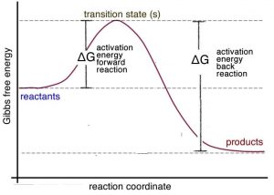
It is important to remember that Le Chatelier’s principle is only a heuristic; it doesn’t tell us why the system shifts to the left. To answer this question, let us consider the energy profile for an exothermic reaction. We can see from the graph \(\rightarrow\) that the activation energy for the reverse (or back) reaction (\(\Delta \mathrm{G} \neq \text{ reverse}\)) is larger than that for the forward reaction (\(\Delta \mathrm{G} \neq \text{ forward}\)). Stated in another way: more energy is required for molecules to react so that the reverse (back) reaction occurs than for the forward reaction. Therefore, it makes sense that if you supply more energy, the reverse reaction is affected more than the forward reaction.^[22]

There is an important difference between disturbing a reaction at equilibrium by changing concentrations of reactants or products, and changing the temperature. When we change the concentrations, the concentrations of all the reactants and products change as the reaction moves towards equilibrium again, but the equilibrium constant stays constant and does not change. However, if we change the temperature, the equilibrium constant changes in value, in a direction that can be predicted by Le Chatelier’s principle.

Equilibrium and Steady State

Now here is an interesting point: imagine a situation in which reactants and products are continually being added to and removed from a system. Such systems are described as open systems, meaning that matter and energy are able to enter or leave them. Open systems are never at equilibrium. Assuming that the changes to the system occur on a time scale that is faster than the rate at which the system returns to equilibrium following a perturbation, the system could well be stable. Such stable, non-equilibrium systems are referred as steady state systems. Think about a cup with a hole in it being filled from a tap. If the rate at which water flows into the cup is equal to the rate at which it flows out, the level of water in the cup would stay the same, even though water would constantly be added to and leave the system (the cup). Living organisms are examples of steady state systems; they are open systems, with energy and matter entering and leaving. However, most equilibrium systems studied in chemistry (at least those discussed in introductory texts) are closed, which means that neither energy nor matter can enter or leave the system.

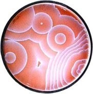
In addition, biological systems are characterized by the fact that there are multiple reactions occurring simultaneously and that a number of these reactions share components—the products of one reaction are the reactants in other reactions. We call this a system of coupled reactions. Such systems can produce quite complex behaviors (as we’ll explore further in Chapter \(9\)). An interesting coupled-reaction system (aside from life itself) is the Belousov–Zhabotinsky (BZ) reaction in which cesium catalyzes the oxidation and bromination of malonic acid.^[23] If the system is not stirred, this reaction can produce quite complex and dynamic spatial patterns, as shown in the figure. The typical BZ reaction involves a closed system, so it will eventually reach a boring (macroscopically-static) equilibrium state. The open nature of biological systems means that complex behaviors do not have to stop; they continue over very long periods of time. The cell theory of life (the theory that all cells are derived from preexisting cells and that all organisms are built from cells or their products), along with the fossil record, indicates that the non-equilibrium system of coupled chemical reactions that has given rise to all organisms has persisted, uninterrupted, for at least \(\sim 3.5\) billion years (a very complex foundation for something as fragile as life).

The steady state systems found in organisms display two extremely important properties: they are adaptive and homeostatic. This means that they can change in response to various stimuli (adaptation) and that they tend to return to their original state following a perturbation (homeostasis). Both are distinct from Le Chatelier’s principle in that they are not passive; they are active processes requiring energy. Adaptation and homeostasis may seem contradictory, but in fact they work together to keep organisms alive and able to adapt to changing conditions.^[24] Even the simplest organisms are characterized by great complexity because of the interconnected and evolved nature of their adaptive and homeostatic systems.

Questions

Questions to Answer

• What does it mean when we say a reaction has reached equilibrium?
• What does the magnitude of the equilibrium constant imply about the extent to which acetic acid ionizes in water?
• Write out the equilibrium constant for the reaction \(\mathrm{H}_{3} \mathrm{O}^{+}+\mathrm{AcO}^{-} \rightleftarrows \mathrm{ACOH}+\mathrm{H}_{2} \mathrm{O}\).
• What would be the value of this equilibrium constant? Does it make sense in terms of what you know about acid-base reactions?
• If the \(\mathrm{pH}\) of a \(0.15-\mathrm{M}\) solution of an acid is \(3.6\), what is the equilibrium constant Ka for this acid? Is the acid a weak or strong acid? How do you know?
• Calcium carbonate (\(\mathrm{CaCO}_{3}\)) is not (very) soluble in water. Write out the equation for the dissolution of \(\mathrm{CaCO}_{3}\). What would be the expression for its \(\mathrm{K}_{eq}\)? (Hint: recall pure solids and liquids do not appear in the expression.) If \(\mathrm{K}_{eq}\) for this process is \(6.0 \times 10^{-9}\), what is the solubility of \(\mathrm{CaCO}_{3}\) in \(\mathrm{mol/L}\)?
• What factors determine the equilibrium concentrations for a reaction?
• For the reaction \(\mathrm{N}_{2}(g)+3 \mathrm{H}_{2}(g) \rightleftarrows 2 \mathrm{NH}_{3}(g)(\Delta \mathrm{H}=-92.4 \mathrm{~kJ} / \mathrm{mol})\), predict the effect on the position of equilibrium, and on the concentrations of all the species in the system, if you:
  • add nitrogen
  • remove hydrogen
  • add ammonia
  • heat the reaction up
  • cool it down
• Draw a reaction energy diagram in which the reverse reaction is much faster than the forward reaction (and vice versa).
• As a system moves towards equilibrium, what is the sign of \(\Delta \mathrm{G}\)? As it moves away from equilibrium, what is the sign of \(\Delta \mathrm{G}\)?
• Explain in your own words the difference between \(\Delta \mathrm{G}^{\circ}\) and \(\Delta \mathrm{G}\).
• Imagine you have a reaction system \(\mathrm{A} \rightleftarrows \mathrm{B}\) for which \(\mathrm{K}_{eq} = 1\). Draw a graph of how \(\Delta \mathrm{G}\) changes as the relative amounts of \([\mathrm{A}]\) and \([\mathrm{B}]\) change.
• What would this graph look like if \(\mathrm{K}_{eq} = 0.1\)? or \(\mathrm{K}_{eq} = 2\)?
• If \(\Delta \mathrm{G}^{\circ}\) is large and positive, what does this mean for the value of \(\mathrm{K}_{eq}\)?
• What if \(\Delta \mathrm{G}^{\circ}\) is large and negative, how does the influence \(\mathrm{K}_{eq}\)?

Questions for Later

• Why is \(\mathrm{K}_{eq}\) temperature-dependent?
• Explain mechanistically why random deviations from equilibrium are reversed.
• If the value of \(\mathrm{Q}\) is \(> \mathrm{K}_{eq}\), what does that tell you about the system? What if \(\mathrm{Q}\) is \(< \mathrm{K}_{eq}\)?

Questions to Ponder

• The acid dissociation constant for ethanol (\(\mathrm{CH}_{3}\mathrm{CH}_{2}\mathrm{OH}\)) is \(\sim 10^{-15}\). Why do you think acetic acid is 10 billion times more acidic than ethanol? (Hint: draw out the structures and think about the stability of the conjugate base.)
• If \(\Delta \mathrm{G}\) for a system is = 0, what does that mean?