26.2: Migration Rates of Solutes

Our ability to separate two solutes depends on the equilibrium interactions of the solute with the stationary phase and the mobile phase, which effects both the time it takes a solute to travel through the column and the width of the solute's elution profile. In this section we consider the rate at which the solute moves through the column.

Distribution Constants

Let’s assume we can describe a solute’s distribution between the mobile phase and stationary phase using the following equilibrium reaction

\[S_{\text{m}} \rightleftharpoons S_{\text{s}} \label{mig1} \]

where S_m is the solute in the mobile phase and S_s is the solute in the stationary phase. The equilibrium constant for this reaction is an equilibrium partition coefficient, K_D.

\[K_{D}=\frac{\left[S_{\mathrm{s}}\right]}{\left[S_\text{m}\right]} \label{mig2} \]

This is not a trivial assumption. In this section we are, in effect, treating the solute’s equilibrium between the mobile phase and the stationary phase as if it is identical to the equilibrium in a simple liquid–liquid extraction carried out in a separatory funnel. You might question whether this is a reasonable assumption. There is an important difference between the two experiments that we need to consider. In a liquid–liquid extraction the two phases remain in contact with each other at all times, allowing for a true equilibrium. In chromatography, however, the mobile phase is in constant motion. A solute that moves into the stationary phase from the mobile phase will equilibrate back into a different portion of the mobile phase; this does not describe a true equilibrium.

So, we ask again: Can we treat a solute’s distribution between the mobile phase and the stationary phase as an equilibrium process? The answer is yes, if the mobile phase velocity is slow relative to the kinetics of the solute’s movement back and forth between the two phase. In general, this is a reasonable assumption.

Retention Time

We can characterize a chromatographic peak’s properties in several ways, two of which are shown in Figure \(\PageIndex{1}\). Retention time, t_r, is the time between the sample’s injection and the maximum response for the solute’s peak. A chromatographic peak’s baseline width, w, as shown in Figure \(\PageIndex{1}\), is determined by extending tangent lines from the inflection points on either side of the peak through the baseline. Although usually we report t_r and w using units of time, we can report them using units of volume by multiplying each by the mobile phase’s velocity, or report them in linear units by measuring distances with a ruler.

For example, a solute’s retention volume,V_r, is \(t_\text{r} \times u\) where u is the mobile phase’s velocity through the column.

Figure \(\PageIndex{1}\). Chromatogram showing a solute’s retention time, t_r, and baseline width, w, and the column’s void time, t_m, for nonretained solutes. In this section we focus on retention time; we will consider the width of the solute's peak in Section 26.3.

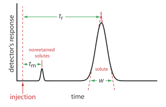
In addition to the solute’s peak, Figure \(\PageIndex{1}\) also shows a small peak that elutes shortly after the sample is injected into the mobile phase. This peak contains all nonretained solutes, which move through the column at the same rate as the mobile phase. The time required to elute the nonretained solutes is called the column’s void time, t_m.

The Rate of Solute Migration: The Retention Factor

In the absence of any additional equilibrium reactions in the mobile phase or the stationary phase, K_D is equivalent to the distribution ratio, D,

\[D=\frac{\left[S_{0}\right]}{\left[S_\text{m}\right]}=\frac{(\operatorname{mol} \text{S})_\text{s} / V_\text{s}}{(\operatorname{mol} \text{S})_\text{m} / V_\text{m}}=K_{D} \label{mig3} \]

where V_s and V_m are the volumes of the stationary phase and the mobile phase, respectively.

A conservation of mass requires that the total moles of solute remain constant throughout the separation; thus, we know that the following equation is true.

\[(\operatorname{mol} \text{S})_{\operatorname{tot}}=(\operatorname{mol} \text{S})_{\mathrm{m}}+(\operatorname{mol} \text{S})_\text{s} \label{mig4} \]

Solving Equation \ref{mig4} for the moles of solute in the stationary phase and substituting into Equation \ref{mig2} leaves us with

\[D = \frac{\left\{(\text{mol S})_{\text{tot}} - (\text{mol S})_\text{m}\right\} / V_{\mathrm{s}}}{(\text{mol S})_{\mathrm{m}} / V_{\mathrm{m}}} \label{mig5} \]

Rearranging this equation and solving for the fraction of solute in the mobile phase, f_m, gives

\[f_\text{m} = \frac {(\text{mol S})_\text{m}} {(\text{mol S})_\text{tot}} = \frac {V_\text{m}} {DV_\text{s} + V_\text{m}} \label{mig6} \]

Because we may not know the exact volumes of the stationary phase and the mobile phase, we simplify Equation \ref{mig6} by dividing both the numerator and the denominator by V_m; thus

\[f_\text{m} = \frac {V_\text{m}/V_\text{m}} {DV_\text{s}/V_\text{m} + V_\text{m}/V_\text{m}} = \frac {1} {DV_\text{s}/V_\text{m} + 1} = \frac {1} {1+k} \label{mig7} \]

where k

\[k=D \times \frac{V_\text{s}}{V_\text{m}} \label{mig8} \]

is the solute’s retention factor. Note that the larger the retention factor, the more the distribution ratio favors the stationary phase, leading to a more strongly retained solute and a longer retention time.

Other (older) names for the retention factor are capacity factor, capacity ratio, and partition ratio, and it sometimes is given the symbol \(k^{\prime}\). Keep this in mind if you are using other resources. Retention factor is the approved name from the IUPAC Gold Book.

We can determine a solute’s retention factor from a chromatogram by measuring the column’s void time, t_m, and the solute’s retention time, t_r (see Figure \(\PageIndex{1}\)). Solving Equation \ref{mig7} for k, we find that

\[k=\frac{1-f_\text{m}}{f_\text{m}} \label{mig9} \]

Earlier we defined f_m as the fraction of solute in the mobile phase. Assuming a constant mobile phase velocity, we also can define f_m as

\[f_\text{m}=\frac{\text { time spent in the mobile phase }}{\text { time spent in the stationary phase }}=\frac{t_\text{m}}{t_\text{r}} \label{mig10} \]

Substituting back into Equation \ref{mig9} and rearranging leaves us with

\[k=\frac{1-\frac{t_{m}}{t_{r}}}{\frac{t_{\mathrm{m}}}{t_{\mathrm{r}}}}=\frac{t_{\mathrm{r}}-t_{\mathrm{m}}}{t_{\mathrm{m}}}=\frac{t_{\mathrm{r}}^{\prime}}{t_{\mathrm{m}}} \label{mig11} \]

where \(t_\text{r}^{\prime}\) is the adjusted retention time.

Example \(\PageIndex{1}\)

In a chromatographic analysis of low molecular weight acids, butyric acid elutes with a retention time of 7.63 min. The column’s void time is 0.31 min. Calculate the retention factor for butyric acid.

Solution

\[k_{\mathrm{but}}=\frac{t_{\mathrm{r}}-t_{\mathrm{m}}}{t_{\mathrm{m}}}=\frac{7.63 \text{ min}-0.31 \text{ min}}{0.31 \text{ min}}=23.6 \nonumber \]

Figure \(\PageIndex{2}\). Chromatogram for Exercise \(\PageIndex{1}\).

Relative Migration Rates: The Selectivity Factor

Selectivity is a relative measure of the retention of two solutes, which we define using a selectivity factor, \(\alpha\)

\[\alpha=\frac{k_{B}}{k_{A}}=\frac{t_{r, B}-t_{\mathrm{m}}}{t_{r, A}-t_{\mathrm{m}}} \label{mig12} \]

where solute A has the smaller retention time. When two solutes elute with identical retention time, \(\alpha = 1.00\); for all other conditions \(\alpha > 1.00\).

Example \(\PageIndex{2}\)

In the chromatographic analysis for low molecular weight acids described in Example \(\PageIndex{1}\), the retention time for isobutyric acid is 5.98 min. What is the selectivity factor for isobutyric acid and butyric acid?

Solution

First we must calculate the retention factor for isobutyric acid. Using the void time from Example \(\PageIndex{1}\) we have

\[k_{\mathrm{iso}}=\frac{t_{\mathrm{r}}-t_{\mathrm{m}}}{t_{\mathrm{m}}}=\frac{5.98 \text{ min}-0.31 \text{ min}}{0.31 \text{ min}}=18.3 \nonumber \]

The selectivity factor, therefore, is

\[\alpha=\frac{k_{\text {but }}}{k_{\text {iso }}}=\frac{23.6}{18.3}=1.29 \nonumber \]