26.3: Zone Broadening and Column Efficiency

Suppose we inject a sample that has a single component. At the moment we inject the sample it is a narrow band of finite width. As the sample passes through the column, the width of this band continually increases in a process we call band broadening. Column efficiency is a quantitative measure of the extent of band broadening.

The Shape of Chromatographic Peaks

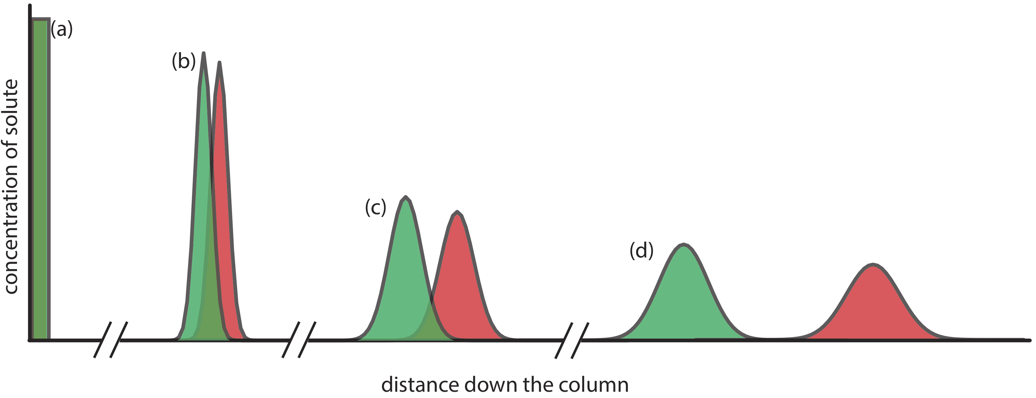
When we inject a sample onto a column it has a uniform, or rectangular concentration profile with respect to distance down the column. As the sample passes through the column, the individual solute particles move in and out of the stationary phase, remaining in place when in the stationary phase and moving down the column when in the mobile phase. Because some solute particles will, on average, spend more time in the mobile phase and some will, on average, spend more time in the stationary phase, the original rectangular band increases in width and takes on a Gaussian shape, as we see in Figure \(\PageIndex{1}\).

Figure \(\PageIndex{1}\). The initial injection of a sample results in the rectangular band of solutes seen in (a). As the sample migrates through the column, the individual components of the sample take on a Gaussian-shaped band profile, as seen in (b-d).

Our treatment of chromatography in this section assumes that a solute elutes as a symmetrical Gaussian peak, such as that shown in Figure \(\PageIndex{1}\). This ideal behavior occurs when the solute’s partition coefficient, K_D

\[K_{\mathrm{D}}=\frac{[S_\text{s}]}{\left[S_\text{m}\right]} \label{shape1} \]

is the same for all concentrations of solute. If this is not the case, then the chromatographic peak has an asymmetric peak shape similar to those shown in Figure \(\PageIndex{2}\). The chromatographic peak in Figure \(\PageIndex{2}\)a is an example of peak tailing, which occurs when some sites on the stationary phase retain the solute more strongly than other sites. Figure \(\PageIndex{2}\)b, which is an example of peak fronting most often is the result of overloading the column with sample.

Figure \(\PageIndex{2}\). Examples of asymmetric chromatographic peaks showing (a) peak tailing and (b) peak fronting. For both (a) and (b) the green chromatogram is the asymmetric peak and the red dashed chromatogram shows the ideal, Gaussian peak shape. The insets show the relationship between the concentration of solute in the stationary phase, [S]_s, and its concentration in the mobile phase, [S]_m. The dashed red lines show ideal behavior (K_D is constant for all conditions) and the green lines show nonideal behavior (K_D decreases or increases for higher total concentrations of solute). A quantitative measure of peak tailing, T, is shown in (a).

As shown in Figure \(\PageIndex{2}\)a, we can report a peak’s asymmetry by drawing a horizontal line at 10% of the peak’s maximum height and measuring the distance from each side of the peak to a line drawn vertically through the peak’s maximum. The asymmetry factor, T, is defined as

\[T=\frac{b}{a} \label{shape2} \]

Methods for Describing Column Efficiency

In their original theoretical model of chromatography, Martin and Synge divided the chromatographic column into discrete sections, which they called theoretical plates. Within each theoretical plate Martin and Synge assumed that there is an equilibrium between the solute present in the stationary phase and the solute present in the mobile phase [Martin, A. J. P.; Synge, R. L. M. Biochem. J. 1941, 35, 1358–1366]. They described column efficiency in terms of the number of theoretical plates, N,

\[N=\frac{L}{H} \label{eff1} \]

where L is the column’s length and H is the height of a theoretical plate. For any given column, the column efficiency improves—and chromatographic peaks become narrower—when there are more theoretical plates.

If we assume that a chromatographic peak has a Gaussian profile, then the extent of band broadening is given by the peak’s variance or standard deviation. The height of a theoretical plate is the peak’s variance per unit length of the column

\[H=\frac{\sigma^{2}}{L} \label{eff2} \]

where the standard deviation, \(\sigma\), has units of distance. Because retention times and peak widths usually are measured in seconds or minutes, it is more convenient to express the standard deviation in units of time, \(\tau\), by dividing \(\sigma\) by the solute’s average linear velocity, \(\overline{u}\), which is equivalent to dividing the distance it travels, L, by its retention time, t_r.

\[\tau=\frac{\sigma}{\overline{u}}=\frac{\sigma t_{r}}{L} \label{eff3} \]

For a Gaussian peak shape, the width at the baseline, w, is four times its standard deviation, \(\tau\).

\[w = 4 \tau \label{eff4} \]

Combining Equation \ref{eff2}, Equation \ref{eff3}, and Equation \ref{eff4} defines the height of a theoretical plate in terms of the easily measured chromatographic parameters t_r and w.

\[H=\frac{L w^{2}}{16 t_\text{r}^{2}} \label{eff5} \]

Combing Equation \ref{eff5} and Equation \ref{eff1} gives the number of theoretical plates.

\[N=16 \frac{t_{\mathrm{r}}^{2}}{w^{2}}=16\left(\frac{t_{\mathrm{r}}}{w}\right)^{2} \label{eff6} \]

Example \(\PageIndex{4}\)

A chromatographic analysis for the chlorinated pesticide Dieldrin gives a peak with a retention time of 8.68 min and a baseline width of 0.29 min. Calculate the number of theoretical plates? Given that the column is 2.0 m long, what is the height of a theoretical plate in mm?

Solution

Using Equation \ref{eff6}, the number of theoretical plates is

\[N=16 \frac{t_{\mathrm{r}}^{2}}{w^{2}}=16 \times \frac{(8.68 \text{ min})^{2}}{(0.29 \text{ min})^{2}}=14300 \text{ plates} \nonumber \]

Solving Equation \ref{eff1} for H gives the average height of a theoretical plate as

\[H=\frac{L}{N}=\frac{2.00 \text{ m}}{14300 \text{ plates}} \times \frac{1000 \text{ mm}}{\mathrm{m}}=0.14 \text{ mm} / \mathrm{plate} \nonumber \]

It is important to remember that a theoretical plate is an artificial construct and that a chromatographic column does not contain physical plates. In fact, the number of theoretical plates depends on both the properties of the column and the solute. As a result, the number of theoretical plates for a column may vary from solute to solute.

The number of theoretical plates for an asymmetric peak shape is approximately

\[N \approx \frac{41.7 \times \frac{t_{r}^{2}}{\left(w_{0.1}\right)^{2}}}{T+1.25}=\frac{41.7 \times \frac{t_{r}^{2}}{(a+b)^{2}}}{T+1.25} \label{eff7} \]

where w_0.1 is the width at 10% of the peak’s height [Foley, J. P.; Dorsey, J. G. Anal. Chem. 1983, 55, 730–737].

Asymmetric peaks have fewer theoretical plates, and the more asymmetric the peak the smaller the number of theoretical plates. For example, the following table gives values for N for a solute eluting with a retention time of 10.0 min and a peak width of 1.00 min.

b	a	T	N
0.5	0.5	1.00	1850
0.6	0.4	1.50	1520
0.7	0.3	2.33	1160
0.8	0.2	4.00	790

Kinetic Variables That Affect Zone Broadening

Another approach to understanding the broadening of a solute band as it passes through a column is to consider the factors that affect the rate at which a solute moves through the column and how that is affected by the velocity with which the mobile phase moves through the column. We will consider one approach that considers four contributions: variations in path lengths, longitudinal diffusion, mass transfer in the stationary phase, and mass transfer in the mobile phase.

Multiple Paths: Variations in Path Length

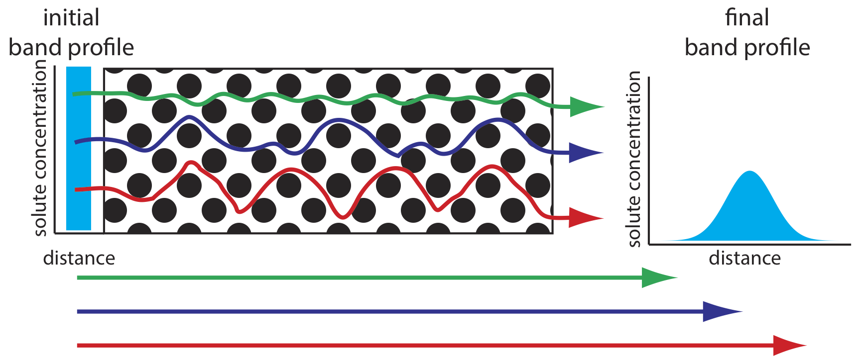
As solute molecules pass through the column they travel paths that differ in length. Because of this difference in path length, two solute molecules that enter the column at the same time will exit the column at different times. The result, as shown in Figure \(\PageIndex{3}\), is a broadening of the solute’s profile on the column. The contribution of multiple paths to the height of a theoretical plate, H_p, is

\[H_{p}=2 \lambda d_{p} \label{van1} \]

where d_p is the average diameter of the particulate packing material and \(\lambda\) is a constant that accounts for the consistency of the packing. A smaller range of particle sizes and a more consistent packing produce a smaller value for \(\lambda\). For a column without packing material, H_p is zero and there is no contribution to band broadening from multiple paths.

Figure \(\PageIndex{3}\). The effect of multiple paths on a solute’s band broadening. The solute’s initial band profile is rectangular. As this band travels through the column, individual solute molecules travel different paths, three of which are shown by the meandering colored paths (the actual lengths of these paths are shown by the straight arrows at the bottom of the figure). Most solute molecules travel paths with lengths similar to that shown in blue, with a few traveling much shorter paths (green) or much longer paths (red). As a result, the solute’s band profile at the end of the column is broader and Gaussian in shape.

An inconsistent packing creates channels that allow some solute molecules to travel quickly through the column. It also can creates pockets that temporarily trap some solute molecules, slowing their progress through the column. A more uniform packing minimizes these problems.

Longitudinal Diffusion

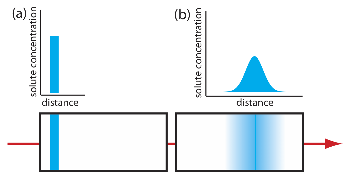
The second contribution to band broadening is the result of the solute’s longitudinal diffusion in the mobile phase. Solute molecules are in constant motion, diffusing from regions of higher solute concentration to regions where the concentration of solute is smaller. The result is an increase in the solute’s band width (Figure \(\PageIndex{4}\)). The contribution of longitudinal diffusion to the height of a theoretical plate, H_d, is

\[H_{d}=\frac{2 \gamma D_{m}}{u} \label{van2} \]

where D_m is the solute’s diffusion coefficient in the mobile phase, u is the mobile phase’s velocity, and \(\gamma\) is a constant related to the efficiency of column packing. Note that the effect of H_d on band broadening is inversely proportional to the mobile phase velocity: a higher velocity provides less time for longitudinal diffusion. Because a solute’s diffusion coefficient is larger in the gas phase than in a liquid phase, longitudinal diffusion is a more serious problem in gas chromatography.

Figure \(\PageIndex{4}\). The effect of longitudinal diffusion on a solute’s band broadening. Two horizontal cross-sections through the column and the corresponding concentration versus distance profiles are shown, with (a) being earlier in time. The red arrow shows the direction in which the mobile phase is moving.

Mass Transfer

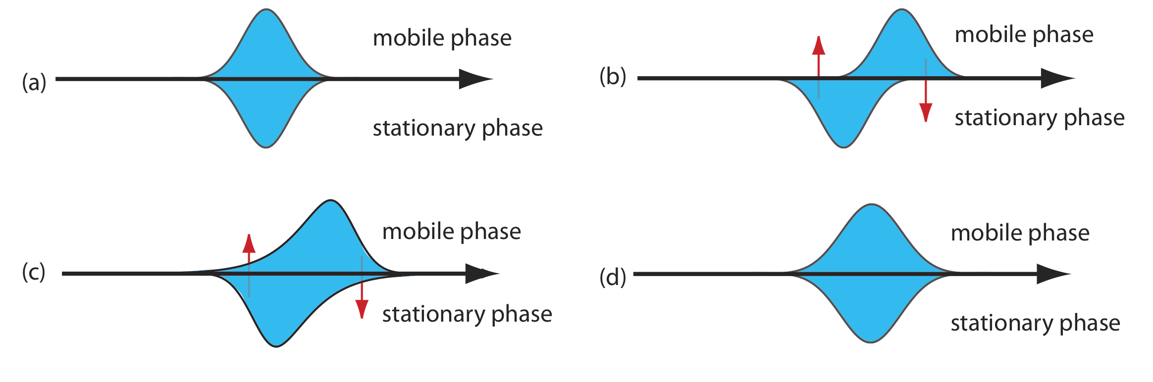
As the solute passes through the column it moves between the mobile phase and the stationary phase. We call this movement between phases mass transfer. As shown in Figure \(\PageIndex{5}\), band broadening occurs if the solute’s movement within the mobile phase or within the stationary phase is not fast enough to maintain an equilibrium in its concentration between the two phases. On average, a solute molecule in the mobile phase moves some distance down the column before it passes into the stationary phase. A solute molecule in the stationary phase, on the other hand, takes longer than expected to move back into the mobile phase. The contributions of mass transfer in the stationary phase, H_s, and mass transfer in the mobile phase, H_m, are given by the following equations

\[H_{s}=\frac{q k d_{f}^{2}}{(1+k)^{2} D_{s}} u \label{van3} \]

\[H_{m}=\frac{f n\left(d_{p}^{2}, d_{c}^{2}\right)}{D_{m}} u \label{van4} \]

where d_f is the thickness of the stationary phase, d_c is the diameter of the column, D_s and D_m are the diffusion coefficients for the solute in the stationary phase and the mobile phase, k is the solute’s retention factor, and q is a constant related to the column packing material. Although the exact form of H_m is not known, it is a function of particle size and column diameter. Note that the effect of H_s and H_m on band broadening is directly proportional to the mobile phase velocity because a smaller velocity provides more time for mass transfer.

The abbreviation fn in Equation \ref{van4} means “is a function of.”

Figure \(\PageIndex{5}\). Effect of mass transfer on band broadening: (a) Ideal equilibrium Gaussian profiles for the solute in the mobile phase and in the stationary phase. (b, c) If we allow the solute’s band to move a small distance down the column, an equilibrium between the two phases no longer exits. The red arrows show the movement of solute—what we call the mass transfer of solute—from the stationary phase to the mobile phase, and from the mobile phase to the stationary phase. (d) Once equilibrium is reestablished, the solute’s band is now broader.

Putting It All Together

The height of a theoretical plate is a summation of the contributions from each of the terms that affect band broadening.

\[H=H_{p}+H_{d}+H_{s}+H_{m} \label{van5} \]

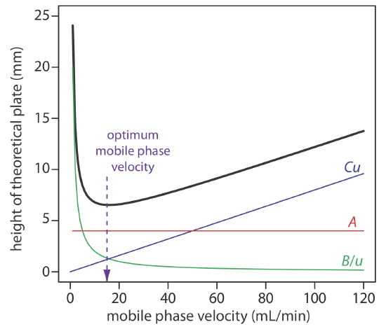
An alternative form of this equation is the van Deemter equation

\[H=A+\frac{B}{u}+C u \label{van6} \]

which emphasizes the importance of the mobile phase’s velocity. In the van Deemter equation, A accounts for the contribution of multiple paths (H_p), B/u accounts for the contribution of longitudinal diffusion (H_d), and Cu accounts for the combined contribution of mass transfer in the stationary phase and in the mobile phase (H_s and H_m).

There is some disagreement on the best equation for describing the relationship between plate height and mobile phase velocity [Hawkes, S. J. J. Chem. Educ. 1983, 60, 393–398]. In addition to the van Deemter equation, other equations include

\[H=\frac{B}{u}+\left(C_s+C_{m}\right) u \label{van7} \]

where C_s and C_m are the mass transfer terms for the stationary phase and the mobile phase and

\[H=A u^{1 / 3}+\frac{B}{u}+C u \label{van8} \]

All three equations, and others, have been used to characterize chromatographic systems, with no single equation providing the best explanation in every case [Kennedy, R. T.; Jorgenson, J. W. Anal. Chem. 1989, 61, 1128–1135].

To increase the number of theoretical plates without increasing the length of the column, we need to decrease one or more of the terms in Equation \ref{van5}. The easiest way to decrease H is to adjust the velocity of the mobile phase. For smaller mobile phase velocities, column efficiency is limited by longitudinal diffusion, and for higher mobile phase velocities efficiency is limited by the two mass transfer terms. As shown in Figure 26.3.6 —which uses the van Deemter equation—the optimum mobile phase velocity is the minimum in a plot of H as a function of u.

Figure 26.3.6 . Plot showing the relationship between the height of a theoretical plate, H, and the mobile phase’s velocity, u, based on the van Deemter equation.

The remaining parameters that affect the terms in Equation \ref{van5} are functions of the column’s properties and suggest other possible approaches to improving column efficiency. For example, both H_p and H_m are a function of the size of the particles used to pack the column. Decreasing particle size, therefore, is another useful method for improving efficiency.

For a more detailed discussion of ways to assess the quality of a column, see Desmet, G.; Caooter, D.; Broeckhaven, K. “Graphical Data Represenation Methods to Assess the Quality of LC Columns,” Anal. Chem. 2015, 87, 8593–8602.

Perhaps the most important advancement in chromatography columns is the development of open-tubular, or capillary columns. These columns have very small diameters (d_c ≈ 50–500 μm) and contain no packing material (d_p = 0). Instead, the capillary column’s interior wall is coated with a thin film of the stationary phase. Plate height is reduced because the contribution to H from H_p (Equation \ref{van1}) disappears and the contribution from H_m (Equation \ref{van4}) becomes smaller. Because the column does not contain any solid packing material, it takes less pressure to move the mobile phase through the column, which allows for longer columns. The combination of a longer column and a smaller height for a theoretical plate increases the number of theoretical plates by approximately \(100 \times\). Capillary columns are not without disadvantages. Because they are much narrower than packed columns, they require a significantly smaller amount of sample, which may be difficult to inject reproducibly. Another approach to improving resolution is to use thin films of stationary phase, which decreases the contribution to H from H_s (Equation \ref{van3}).

The smaller the particles, the more pressure is needed to push the mobile phase through the column. As a result, for any form of chromatography there is a practical limit to particle size.