1.4: Selecting an Analytical Method

The analysis of a sample generates a chemical or a physical signal that is proportional to the amount of analyte in the sample. This signal may be anything we can measure, such the examples described in Section 1.2. It is convenient to divide analytical techniques into two general classes based on whether the signal is directly proportional to the mass or moles of analyte, or is directly proportional to the analyte’s concentration.

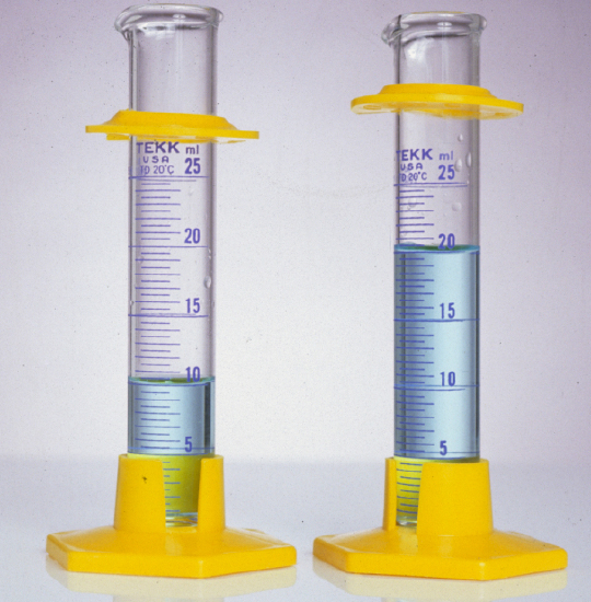
Consider the two graduated cylinders in Figure \(\PageIndex{1}\), each of which contains a solution of 0.010 M Cu(NO₃)₂. The cylinder on the left contains 10 mL, or \(1.0 \times 10^{-4}\) moles of Cu²⁺, and the cylinder on the right contains 20 mL, or \(2.0 \times 10^{-4}\) moles of Cu²⁺. If a technique responds to the absolute amount of analyte in the sample, then the signal due to the analyte S_A is given as

\[S_A = k_A n_A \label{totalanalysis} \]

where n_A is the moles or grams of analyte in the sample, and k_A is a proportionality constant. Because the cylinder on the right contains twice as many moles of Cu²⁺ as the cylinder on the left, analyzing its contents gives a signal twice as large as that for the other cylinder.

Figure \(\PageIndex{1}\): Two graduated cylinders, each containing 0.10 M Cu(NO₃)₂. Although the cylinders contain the same concentration of Cu²⁺, the cylinder on the left contains \(1.0 \times 10^{-4}\) mol Cu²⁺ and the cylinder on the right contains \(2.0 \times 10^{-4}\) mol Cu²⁺.

A second class of analytical techniques are those that respond to the analyte’s concentration, C_A

\[S_A = k_A C_A \label{concanalysis} \]

In this case, an analysis of the contents of the two cylinders gives the same result. As most instruments respond to the analyte's concentration, we will imit ourselves to using Equation \ref{concanalysis} for the remainder of this section.

Defining the Problem

To select an appropriate analytical method for a particular problem we need to consider our needs and compare them to the strengths and weaknesses of the available analytical methods. If we are screening samples on a production line to determine if an analyte exceeds a threshold so that we can set them aside for a more careful analysis, then we may wish to give more consideration to speed than to accuracy or precision. On the other hand, if we our analyte is part of a complex mixture, then we may wish to give more consideration to analytical methods that provide for greater selectivity. Or, if we expect that our samples will vary substantially in the concentration of analyte, then we may give more consideration to an analytical method for which Equation \ref{concanalysis} applies over a wide range of concentrations.

Performance Characteristics of Instruments

As suggested above, when we choose an analytical method, we match the its performance characteristics (or figures of merit) to our needs. Some of these characteristics are quantitative (accuracy, precision, sensitivity, detection limit, selectivity, dynamic range, and selectivity) and others are more qualitative (robustness, ruggedness, scale of operation, time, and cost).

Accuracy

Accuracy, or bias, is a measure of how close the result of an experiment is to the “true” or expected result. We can express accuracy as an absolute error, e

\[e = x - \mu \nonumber \]

where \(x\) is the experimental result and \(\mu\) is the expected result, or as a percentage relative error, %e_r

\[\% e_r = \frac {x - \mu} {\mu} \times 100 \nonumber \]

A method’s accuracy depends on many things, including the signal’s source, the value of k_A in Equation \ref{concanalysis}, and the ease of handling samples without loss or contamination.

Because it is unlikely that we know the true result, we can use an expected or accepted result to evaluate accuracy. For example, we might use a standard reference material, which has an accepted value for our analyte, to establish the analytical method’s accuracy. You will find a more detailed treatment of accuracy in, including a discussion of sources of errors, in Appendix 1.

Precision

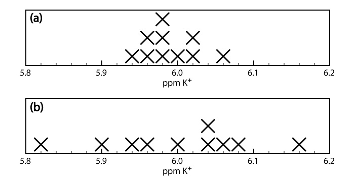
When we analyze a sample several times, the individual results vary from trial-to-trial. Precision is a measure of this variability. The closer the agreement between individual analyses, the more precise the results. For example, the results shown in the upper half of Figure \(\PageIndex{2}\) for the concentration of potassium in a sample of serum are more precise than those in the lower half of Figure \(\PageIndex{2}\). It is important to understand that precision does not imply accuracy. That the data in the upper half of Figure \(\PageIndex{2}\) are more precise does not mean that the first set of results is more accurate. In fact, neither set of results may be accurate.

Figure \(\PageIndex{2}\): Two determinations of the concentration of potassium in serum, showing the effect of precision on the distribution of individual results. The data in (a) are less scattered and, therefore, more precise than the data in (b).

A method’s precision depends on several factors, including the uncertainty in measuring the signal and the ease of handling samples reproducibly, and is reported as an absolute standard deviation, s

\[s = \sqrt{\frac {\sum_{i = 1}^{n} (X_i - \overline{X})^{2}} {n - 1}} \label{sd} \]

or a relative standard deviation, s_r

\[s_r = \frac {s} {\overline{X}} \label{rsd} \]

where \(\overline{X}\) is the average, or mean value of the individual measurements.

\[\overline{X} = \frac {\sum_{i = 1}^n X_i} {n} \label{mean} \]

Confusing accuracy and precision is a common mistake. See Ryder, J.; Clark, A. U. Chem. Ed. 2002, 6, 1–3, and Tomlinson, J.; Dyson, P. J.; Garratt, J. U. Chem. Ed. 2001, 5, 16–23 for discussions of this and other common misconceptions about the meaning of error. You will find a more detailed treatment of precision in Appendix 1, including a discussion of sources of errors.

Sensitivity

The ability to demonstrate that two samples have different amounts of analyte is an essential part of many analyses. A method’s sensitivity is a measure of its ability to establish that such a difference is significant. Sensitivity is often confused with a method’s detection limit, which is the smallest amount of analyte we can determine with confidence.

See Pardue, H. L. Clin. Chem. 1997, 43, 1831-1837 for an explanation for why a method's sensitivity is not the same as its detection limit.

Sensitivity is equivalent to the proportionality constant, k_A, in Equation \ref{concanalysis} [IUPAC Compendium of Chemical Terminology, Electronic version]. If \(\Delta S_A\) is the smallest difference we can measure between two signals, then the smallest detectable difference in the analyte's concentration is

\[\Delta C_A = \frac {\Delta S_A} {k_A} \nonumber \]

Suppose, for example, that our analytical signal is a measurement for which the smallest detectable increment is ±0.001 (arbitrary units). If our method’s sensitivity is \(0.200 \text{M}^{-1}\), then our method can conceivably detect a difference in concentration of as little as

\[\Delta C_A = \frac {\pm 0.001 } {0.200 \text{ M}^{-1}} = \pm 0.005 \text{ M}^{-1} \nonumber \]

For two methods with the same \(\Delta S_A\), the method with the greater sensitivity—that is, the method with the larger k_A—is better able to discriminate between smaller amounts of analyte.

Detection Limit

The International Union of Pure and Applied Chemistry (IUPAC) defines a method’s detection limit as the smallest concentration or absolute amount of analyte that has a signal significantly larger than the signal from a suitable blank [IUPAC Compendium of Chemical Technology, Electronic Version]. Although our interest is in the amount of analyte, in this section we will define the detection limit in terms of the analyte’s signal. Knowing the signal, we can calculate the analyte’s concentration, C_A, using Equation \ref{concanalysis}, \(S_A = k_A C_A\) where k is the method’s sensitivity.

Let’s translate the IUPAC definition of the detection limit into a mathematical form by letting S_mb represent the average signal for a method blank, and letting \(\sigma_{mb}\) represent the method blank’s standard deviation. To detect the analyte, its signal must exceed S_mb by a suitable amount; thus,

\[(S_A)_{DL} = S_{mb} \pm z \sigma_{mb} \label{detlimit} \]

where \((S_A)_{DL}\) is the analyte’s detection limit.

The value we choose for z depends on our tolerance for reporting the analyte’s concentration even if it is absent from the sample (what is called a type 1 error). Typically, z is set to three, which corresponds to a probability, \(\alpha\), of 0.00135, or 0.135%. As shown in Figure \(\PageIndex{3}\)a, there is only a 0.135% probability of detecting the analyte in a sample that actually is analyte-free.

Figure \(\PageIndex{3}\): Normal distribution curves showing the probability of type 1 and type 2 errors for the IUPAC detection limit. (a) The normal distribution curve for the method blank, with S_mb = 0 and \(\sigma_{mb}\) = 1. The minimum detectable signal for the analyte, (S_A)_DL, has a type 1 error of 0.135%. (b) The normal distribution curve for the analyte at its detection limit, (S_A)_DL= 3, is superimposed on the normal distribution curve for the method blank. The standard deviation for the analyte’s signal, \(\sigma_A\), is 0.8, The area in green represents the probability of a type 2 error, which is 50%. The inset shows, in blue, the probability of a type 1 error, which is 0.135%.

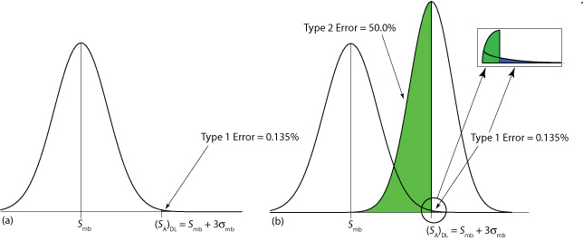
A detection limit also is subject to a type 2 error in which we fail to find evidence for the analyte even though it is present in the sample. Consider, for example, the situation shown in Figure \(\PageIndex{3}\)b where the signal for a sample that contains the analyte is exactly equal to (S_A)_DL. In this case the probability of a type 2 error is 50% because half of the sample’s possible signals are below the detection limit. We correctly detect the analyte at the IUPAC detection limit only half the time. The IUPAC definition for the detection limit is the smallest signal for which we can say, at a significance level of \(\alpha\), that an analyte is present in the sample; however, failing to detect the analyte does not mean it is not present in the sample.

The detection limit often is represented, particularly when discussing public policy issues, as a distinct line that separates detectable concentrations of analytes from concentrations we cannot detect. This use of a detection limit is incorrect [Rogers, L. B. J. Chem. Educ. 1986, 63, 3–6]. As suggested by Figure \(\PageIndex{3}\), for an analyte whose concentration is near the detection limit there is a high probability that we will fail to detect the analyte.

An alternative expression for the detection limit, the limit of identification, minimizes both type 1 and type 2 errors [Long, G. L.; Winefordner, J. D. Anal. Chem. 1983, 55, 712A–724A]. The analyte’s signal at the limit of identification, (S_A)_LOI, includes an additional term, \(z \sigma_A\), to account for the distribution of the analyte’s signal.

\[(S_A)_\text{LOI} = (S_A)_\text{DL} + z \sigma_A = S_{mb} + z \sigma_{mb} + z \sigma_A \label{loi} \]

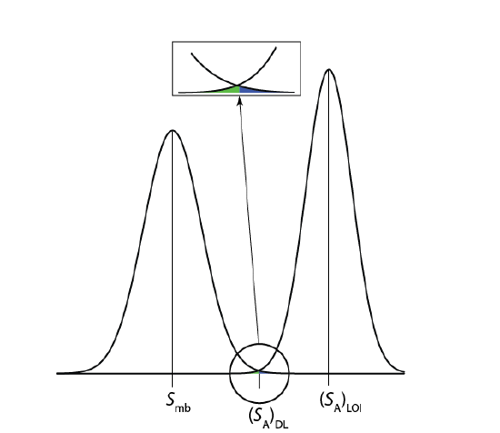
As shown in Figure \(\PageIndex{4}\), the limit of identification provides an equal probability of a type 1 and a type 2 error at the detection limit. When the analyte’s concentration is at its limit of identification, there is only a 0.135% probability that its signal is indistinguishable from that of the method blank.

Figure \(\PageIndex{4}\): Normal distribution curves for a method blank and for a sample at the limit of identification: S_mb = 0; \(\sigma_{mb} = 1\); \(\sigma_A = 0.8\); and (S_A)_LOI = 0 + 3 \(\times\) 1 + 3 \(\times\) 0.8 = 5.4. The inset shows that the probability of a type 1 error (0.135%) is the same as the probability of a type 2 error (0.135%).

The ability to detect the analyte with confidence is not the same as the ability to report with confidence its concentration, or to distinguish between its concentration in two samples. For this reason the American Chemical Society’s Committee on Environmental Analytical Chemistry recommends the limit of quantitation, (S_A)_LOQ [“Guidelines for Data Acquisition and Data Quality Evaluation in Environmental Chemistry,” Anal. Chem. 1980, 52, 2242–2249 ].

\[(S_A)_\text{LOQ} = S_{mb} + 10 \sigma_{mb} \label{loq} \]

Dynamic Range

A method's dynamic range (or linear range) runs from its limit of quantication, (Equation \ref{loq}, to the highest concentration for which the sensitivity, k_A, remains constant, resulting in a straight-line relationship between \(S_A\) and \(C_A\). This upper limit is called the limit of linearity, LOL. Between the LOQ and the LOL we can use Equation \ref{concanalysis} to convert a measured signal into the corresponding concentration of the analyte. Above the LOQ the relationship between the signal and the analyte's concentration no longer is a straight-line.

Selectivity

An analytical method is specific if its signal depends only on the analyte [Persson, B-A; Vessman, J. Trends Anal. Chem. 1998, 17, 117–119; Persson, B-A; Vessman, J. Trends Anal. Chem. 2001, 20, 526–532]. Although specificity is the ideal, few analytical methods are free from interferences. When an interferent, I, contributes to the signal, we expand \ref{totalanalysis} and Equation \ref{concanalysis} to include its contribution to the sample’s signal, S_samp

\[S_{samp} = S_A + S_I = k_A C_A + k_I C_I \label{concsamp} \]

where S_I is the interferent’s contribution to the signal, k_I is the interferent’s sensitivity, and C_I is the concentration of interferent in the sample.

Selectivity is a measure of a method’s freedom from interferences [Valcárcel, M.; Gomez-Hens, A.; Rubio, S. Trends Anal. Chem. 2001, 20, 386–393]. A method’s selectivity for an interferent relative to the analyte is defined by a selectivity coefficient, K_A,I

\[K_{A,I} = \frac {k_I} {k_A} \label{selectcoef} \]

which may be positive or negative depending on the signs of k_I and k_A. The selectivity coefficient is greater than +1 or less than –1 when the method is more selective for the interferent than for the analyte.

Although k_A and k_I usually are positive, they can be negative. For example, some analytical methods work by measuring the concentration of a species that remains after is reacts with the analyte. As the analyte’s concentration increases, the concentration of the species that produces the signal decreases, and the signal becomes smaller. If the signal in the absence of analyte is assigned a value of zero, then the subsequent signals are negative.

Determining the selectivity coefficient’s value is easy if we already know the values for k_A and k_I. As shown by Example \(\PageIndex{1}\), we also can determine K_A,I by measuring S_samp in the presence of and in the absence of the interferent.

Example \(\PageIndex{1}\)

A method for the analysis of Ca²⁺ in water suffers from an interference in the presence of Zn²⁺. When the concentration of Ca²⁺ is 100 times greater than that of Zn²⁺, an analysis for Ca²⁺ has a relative error of +0.5%. What is the selectivity coefficient for this method?

Solution

Since only relative concentrations are reported, we can arbitrarily assign absolute concentrations. To make the calculations easy, we will let C_Ca = 100 (arbitrary units) and C_Zn = 1. A relative error of +0.5% means the signal in the presence of Zn²⁺ is 0.5% greater than the signal in the absence of Zn²⁺. Again, we can assign values to make the calculation easier. If the signal for Cu²⁺ in the absence of Zn²⁺ is 100 (arbitrary units), then the signal in the presence of Zn²⁺ is 100.5.

The value of k_Ca is determined using Equation \ref{concanalysis}

\[k_\text{Ca} = \frac {S_\text{Ca}} {C_\text{Ca}} = \frac {100} {100} = 1 \nonumber \]

In the presence of Zn²⁺ the signal is given by Equation \ref{concsamp}; thus

\[S_{samp} = 100.5 = k_\text{Ca} C_\text{Ca} + k_\text{Zn} C_\text{Zn} = (1 \times 100) + k_\text{Zn} \times 1 \nonumber \]

Solving for k_Zn gives its value as 0.5. The selectivity coefficient is

\[K_\text{Ca,Zn} = \frac {k_\text{Zn}} {k_\text{Ca}} = \frac {0.5} {1} = 0.5 \nonumber \]

If you are unsure why, in the above example, the signal in the presence of zinc is 100.5, note that the percentage relative error for this problem is given by

\[\frac {\text{obtained result} - 100} {100} \times 100 = +0.5 \% \nonumber \]

Solving gives an obtained result of 100.5.

A selectivity coefficient provides us with a useful way to evaluate an interferent’s potential effect on an analysis. Solving Equation \ref{selectcoef} for k_I

\[k_I = K_{A,I} \times k_A \label{ki} \]

and substituting in Equation \ref{concanalysis} and simplifying gives

\[S_{samp} = k_A \{ C_A + K_{A,I} \times C_I \} \label{S_samp} \]

An interferent will not pose a problem as long as the term \(K_{A,I} \times C_I\) in Equation \ref{S_samp} is significantly smaller than than C_A.

Example \(\PageIndex{2}\)

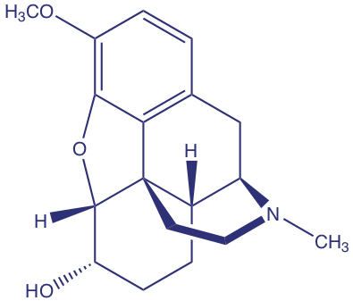
Barnett and colleagues developed a method to determine the concentration of codeine (structure shown below) in poppy plants [Barnett, N. W.; Bowser, T. A.; Geraldi, R. D.; Smith, B. Anal. Chim. Acta 1996, 318, 309– 317]. As part of their study they evaluated the effect of several interferents. For example, the authors found that equimolar solutions of codeine and the interferent 6-methoxycodeine gave signals, respectively of 40 and 6 (arbitrary units).

(a) What is the selectivity coefficient for the interferent, 6-methoxycodeine, relative to that for the analyte, codeine.

(b) If we need to know the concentration of codeine with an accuracy of ±0.50%, what is the maximum relative concentration of 6-methoxy-codeine that we can tolerate?

Solution

(a) The signals due to the analyte, S_A, and the interferent, S_I, are

\[S_A = k_A C_A \quad \quad S_I = k_I C_I \nonumber \]

Solving these equations for k_A and for k_I, and substituting into Equation \ref{selectcoef} gives

\[K_{A,I} = \frac {S_I / C_I} {S_A / C_I} \nonumber \]

Because the concentrations of analyte and interferent are equimolar (C_A = C_I), the selectivity coefficient is

\[K_{A,I} = \frac {S_I} {S_A} = \frac {6} {40} = 0.15 \nonumber \]

(b) To achieve an accuracy of better than ±0.50% the term \(K_{A,I} \times C_I\) in Equation \ref{S_samp} must be less than 0.50% of C_A; thus

\[K_{A,I} \times C_I \le 0.0050 \times C_A \nonumber \]

Solving this inequality for the ratio C_I/C_A and substituting in the value for K_A,I from part (a) gives

\[\frac {C_I} {C_A} \le \frac {0.0050} {K_{A,I}} = \frac {0.0050} {0.15} = 0.033 \nonumber \]

Therefore, the concentration of 6-methoxycodeine must be less than 3.3% of codeine’s concentration.

Problems with selectivity also are more likely when the analyte is present at a very low concentration [Rodgers, L. B. J. Chem. Educ. 1986, 63, 3–6].

Robustness and Ruggedness

For a method to be useful it must provide reliable results. Unfortunately, methods are subject to a variety of chemical and physical interferences that contribute uncertainty to the analysis. If a method is relatively free from chemical interferences, we can use it to analyze an analyte in a wide variety of sample matrices. Such methods are considered robust.

Random variations in experimental conditions introduces uncertainty. If a method’s sensitivity, k, is too dependent on experimental conditions, such as temperature, acidity, or reaction time, then a slight change in any of these conditions may give a significantly different result. A rugged method is relatively insensitive to changes in experimental conditions.

Scale of Operation

Another way to narrow the choice of methods is to consider three potential limitations: the amount of sample available for the analysis, the expected concentration of analyte in the samples, and the minimum amount of analyte that will produce a measurable signal. Collectively, these limitations define the analytical method’s scale of operations.

We can display the scale of operations visually (Figure \(\PageIndex{5}\)) by plotting the sample’s size on the x-axis and the analyte’s concentration on the y-axis. For convenience, we divide samples into macro (>0.1 g), meso (10 mg–100 mg), micro (0.1 mg–10 mg), and ultramicro (<0.1 mg) sizes, and we divide analytes into major (>1% w/w), minor (0.01% w/w–1% w/w), trace (10^–7% w/w–0.01% w/w), and ultratrace (<10^–7% w/w) components. Together, the analyte’s concentration and the sample’s size provide a characteristic description for an analysis. For example, in a microtrace analysis the sample weighs between 0.1 mg and 10 mg and contains a concentration of analyte between 10^–7% w/w and 10^–2% w/w.

Figure \(\PageIndex{5}\): Scale of operations for analytical methods. The shaded areas define different types of analyses. The boxed area, for example, represents a microtrace analysis. The diagonal lines show combinations of sample size and analyte concentration that contain the same mass of analyte. The three filled circles (•), for example, indicate analyses that use 10 mg of analyte. See Sandell, E. B.; Elving, P. J. in Kolthoff, I. M.; Elving, P. J., eds. Treatise on Analytical Chem-istry, Interscience: New York, Part I, Vol. 1, Chapter 1, pp. 3–6; (b) Potts, L. W. Quantitative Analysis–Theory and Practice, Harper and Row: New York, 1987, pp. 12 for more details.

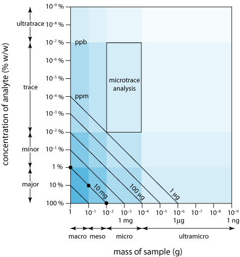
The diagonal lines connecting the axes show combinations of sample size and analyte concentration that contain the same absolute mass of analyte. As shown in Figure \(\PageIndex{5}\), for example, a 1-g sample that is 1% w/w analyte has the same amount of analyte (10 mg) as a 100-mg sample that is 10% w/w analyte, or a 10-mg sample that is 100% w/w analyte.

We can use Figure \(\PageIndex{5}\) to establish limits for analytical methods. If a method’s minimum detectable signal is equivalent to 10 mg of analyte, then it is best suited to a major analyte in a macro or meso sample. Extending the method to an analyte with a concentration of 0.1% w/w requires a sample of 10 g, which rarely is practical due to the complications of carrying such a large amount of material through the analysis. On the other hand, a small sample that contains a trace amount of analyte places significant restrictions on an analysis. For example, a 1-mg sample that is 10^–4% w/w in analyte contains just 1 ng of analyte. If we isolate the analyte in 1 mL of solution, then we need an analytical method that reliably can detect it at a concentration of 1 ng/mL.

Equipment, Time, and Cost

Finally, we can compare analytical methods with respect to their equipment needs, the time needed to complete an analysis, and the cost per sample. Methods that rely on instrumentation are equipment-intensive and may require significant operator training. For example, the graphite furnace atomic absorption spectroscopic method for determining lead in water requires a significant capital investment in the instrument and an experienced operator to obtain reliable results. Other methods, such as titrimetry, require less expensive equipment and less training.

The time to complete an analysis for one sample often is fairly similar from method-to-method. This is somewhat misleading, however, because much of this time is spent preparing samples, preparing reagents, and gathering together equipment. Once the samples, reagents, and equipment are in place, the sampling rate may differ substantially. For example, it takes just a few minutes to analyze a single sample for lead using graphite furnace atomic absorption spectroscopy, but several hours to analyze the same sample using gravimetry. This is a significant factor in selecting a method for a laboratory that handles a high volume of samples.

The cost of an analysis depends on many factors, including the cost of equipment and reagents, the cost of hiring analysts, and the number of samples that can be processed per hour. In general, methods that rely on instruments cost more per sample then other methods.

Making the Final Choice

Unfortunately, the design criteria discussed in this section are not mutually independent [Valcárcel, M.; Ríos, A. Anal. Chem. 1993, 65, 781A–787A]. Working with smaller samples or improving selectivity often comes at the expense of precision. Minimizing cost and analysis time may decrease accuracy. Selecting a method requires carefully balancing the various design criteria. Usually, the most important design criterion is accuracy, and the best method is the one that gives the most accurate result. When the need for a result is urgent, as is often the case in clinical labs, analysis time may become the critical factor.

In some cases it is the sample’s properties that determine the best method. A sample with a complex matrix, for example, may require a method with excellent selectivity to avoid interferences. Samples in which the analyte is present at a trace or ultratrace concentration usually require a concentration method. If the quantity of sample is limited, then the method must not require a large amount of sample.