
1.3: Instruments For Analysis
- Page ID
- 332834

\( \newcommand{\vecs}[1]{\overset { \scriptstyle \rightharpoonup} {\mathbf{#1}} } \)
\( \newcommand{\vecd}[1]{\overset{-\!-\!\rightharpoonup}{\vphantom{a}\smash {#1}}} \)
\( \newcommand{\dsum}{\displaystyle\sum\limits} \)
\( \newcommand{\dint}{\displaystyle\int\limits} \)
\( \newcommand{\dlim}{\displaystyle\lim\limits} \)
\( \newcommand{\id}{\mathrm{id}}\) \( \newcommand{\Span}{\mathrm{span}}\)
( \newcommand{\kernel}{\mathrm{null}\,}\) \( \newcommand{\range}{\mathrm{range}\,}\)
\( \newcommand{\RealPart}{\mathrm{Re}}\) \( \newcommand{\ImaginaryPart}{\mathrm{Im}}\)
\( \newcommand{\Argument}{\mathrm{Arg}}\) \( \newcommand{\norm}[1]{\| #1 \|}\)
\( \newcommand{\inner}[2]{\langle #1, #2 \rangle}\)
\( \newcommand{\Span}{\mathrm{span}}\)
\( \newcommand{\id}{\mathrm{id}}\)
\( \newcommand{\Span}{\mathrm{span}}\)
\( \newcommand{\kernel}{\mathrm{null}\,}\)
\( \newcommand{\range}{\mathrm{range}\,}\)
\( \newcommand{\RealPart}{\mathrm{Re}}\)
\( \newcommand{\ImaginaryPart}{\mathrm{Im}}\)
\( \newcommand{\Argument}{\mathrm{Arg}}\)
\( \newcommand{\norm}[1]{\| #1 \|}\)
\( \newcommand{\inner}[2]{\langle #1, #2 \rangle}\)
\( \newcommand{\Span}{\mathrm{span}}\) \( \newcommand{\AA}{\unicode[.8,0]{x212B}}\)
\( \newcommand{\vectorA}[1]{\vec{#1}} % arrow\)
\( \newcommand{\vectorAt}[1]{\vec{\text{#1}}} % arrow\)
\( \newcommand{\vectorB}[1]{\overset { \scriptstyle \rightharpoonup} {\mathbf{#1}} } \)
\( \newcommand{\vectorC}[1]{\textbf{#1}} \)
\( \newcommand{\vectorD}[1]{\overrightarrow{#1}} \)
\( \newcommand{\vectorDt}[1]{\overrightarrow{\text{#1}}} \)
\( \newcommand{\vectE}[1]{\overset{-\!-\!\rightharpoonup}{\vphantom{a}\smash{\mathbf {#1}}}} \)
\( \newcommand{\vecs}[1]{\overset { \scriptstyle \rightharpoonup} {\mathbf{#1}} } \)
\(\newcommand{\longvect}{\overrightarrow}\)
\( \newcommand{\vecd}[1]{\overset{-\!-\!\rightharpoonup}{\vphantom{a}\smash {#1}}} \)
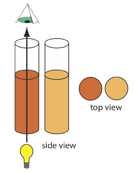
\(\newcommand{\avec}{\mathbf a}\) \(\newcommand{\bvec}{\mathbf b}\) \(\newcommand{\cvec}{\mathbf c}\) \(\newcommand{\dvec}{\mathbf d}\) \(\newcommand{\dtil}{\widetilde{\mathbf d}}\) \(\newcommand{\evec}{\mathbf e}\) \(\newcommand{\fvec}{\mathbf f}\) \(\newcommand{\nvec}{\mathbf n}\) \(\newcommand{\pvec}{\mathbf p}\) \(\newcommand{\qvec}{\mathbf q}\) \(\newcommand{\svec}{\mathbf s}\) \(\newcommand{\tvec}{\mathbf t}\) \(\newcommand{\uvec}{\mathbf u}\) \(\newcommand{\vvec}{\mathbf v}\) \(\newcommand{\wvec}{\mathbf w}\) \(\newcommand{\xvec}{\mathbf x}\) \(\newcommand{\yvec}{\mathbf y}\) \(\newcommand{\zvec}{\mathbf z}\) \(\newcommand{\rvec}{\mathbf r}\) \(\newcommand{\mvec}{\mathbf m}\) \(\newcommand{\zerovec}{\mathbf 0}\) \(\newcommand{\onevec}{\mathbf 1}\) \(\newcommand{\real}{\mathbb R}\) \(\newcommand{\twovec}[2]{\left[\begin{array}{r}#1 \\ #2 \end{array}\right]}\) \(\newcommand{\ctwovec}[2]{\left[\begin{array}{c}#1 \\ #2 \end{array}\right]}\) \(\newcommand{\threevec}[3]{\left[\begin{array}{r}#1 \\ #2 \\ #3 \end{array}\right]}\) \(\newcommand{\cthreevec}[3]{\left[\begin{array}{c}#1 \\ #2 \\ #3 \end{array}\right]}\) \(\newcommand{\fourvec}[4]{\left[\begin{array}{r}#1 \\ #2 \\ #3 \\ #4 \end{array}\right]}\) \(\newcommand{\cfourvec}[4]{\left[\begin{array}{c}#1 \\ #2 \\ #3 \\ #4 \end{array}\right]}\) \(\newcommand{\fivevec}[5]{\left[\begin{array}{r}#1 \\ #2 \\ #3 \\ #4 \\ #5 \\ \end{array}\right]}\) \(\newcommand{\cfivevec}[5]{\left[\begin{array}{c}#1 \\ #2 \\ #3 \\ #4 \\ #5 \\ \end{array}\right]}\) \(\newcommand{\mattwo}[4]{\left[\begin{array}{rr}#1 \amp #2 \\ #3 \amp #4 \\ \end{array}\right]}\) \(\newcommand{\laspan}[1]{\text{Span}\{#1\}}\) \(\newcommand{\bcal}{\cal B}\) \(\newcommand{\ccal}{\cal C}\) \(\newcommand{\scal}{\cal S}\) \(\newcommand{\wcal}{\cal W}\) \(\newcommand{\ecal}{\cal E}\) \(\newcommand{\coords}[2]{\left\{#1\right\}_{#2}}\) \(\newcommand{\gray}[1]{\color{gray}{#1}}\) \(\newcommand{\lgray}[1]{\color{lightgray}{#1}}\) \(\newcommand{\rank}{\operatorname{rank}}\) \(\newcommand{\row}{\text{Row}}\) \(\newcommand{\col}{\text{Col}}\) \(\renewcommand{\row}{\text{Row}}\) \(\newcommand{\nul}{\text{Nul}}\) \(\newcommand{\var}{\text{Var}}\) \(\newcommand{\corr}{\text{corr}}\) \(\newcommand{\len}[1]{\left|#1\right|}\) \(\newcommand{\bbar}{\overline{\bvec}}\) \(\newcommand{\bhat}{\widehat{\bvec}}\) \(\newcommand{\bperp}{\bvec^\perp}\) \(\newcommand{\xhat}{\widehat{\xvec}}\) \(\newcommand{\vhat}{\widehat{\vvec}}\) \(\newcommand{\uhat}{\widehat{\uvec}}\) \(\newcommand{\what}{\widehat{\wvec}}\) \(\newcommand{\Sighat}{\widehat{\Sigma}}\) \(\newcommand{\lt}{<}\) \(\newcommand{\gt}{>}\) \(\newcommand{\amp}{&}\) \(\definecolor{fillinmathshade}{gray}{0.9}\)An early example of a colorimetric analysis is Nessler’s method for ammonia, which was introduced in 1856. Nessler found that adding an alkaline solution of HgI2 and KI to a dilute solution of ammonia produced a yellow-to-reddish brown colloid in which the colloid’s color depended on the concentration of ammonia. In addition to the sample, Nessler prepared a series of standard solutions, each containing a known amount of ammonia, and placed each in a glass tube with a flat bottom. Allowing sunlight to pass through the tubes from bottom-to-top, Nessler observed them from above, as seen in Figure \(\PageIndex{1}\). By visually comparing the color of the sample to the colors of the standards, Nessler was able to estimate the concentration of ammonia in the sample.
Nessler's method converts a sample's chemical and/or physical properties—the color that forms when NH3 reacts with HgI2 and KI—into a signal that we can detect, process, and report as a relative measure of the amount of NH3 in the sample. Although we might not think of a Nessler tube as an instrument, the process of probing a sample in a way that converts its chemical or physical properties into a form of information that we can report is the essence of any instrument.
The basic components of an instrument include a probe that interacts with the sample, an input transducer that converts the sample's chemical and/or physical properties into an electrical signal, a signal processor that converts the electrical signal into a form that an output transducer can convert into a numerical or visual output that we can understand. We can represent this as a sequence of actions that take place within the instrument
\[\text{probe} \rightarrow \text{sample} \rightarrow \text{input transducer} \rightarrow \text{raw data} \rightarrow \text{signal processor} \rightarrow \text{output transducer} \nonumber \]
and as a general flow of information
\[\text{chemical and/or physical information} \rightarrow \text{electrical information} \rightarrow \text{numerical or visual response} \nonumber \]
In Nessler’s method, the probe is sunlight, the analyst’s eye is the input transducer, the raw data is the response of the eye's optic nerve to the attenuation of light, the signal processor is the brain, and the output is a visual report of the sample's color relative to the standards.
\[\text{sunlight} \rightarrow \text{sample} \rightarrow \text{eye} \rightarrow \text{response of optic nerve} \rightarrow \text{brain} \rightarrow \text{visual report of color} \nonumber \]
Ways to Encode Information
As suggested above, information is encoded in two broad ways: as electrical information (such as currents and potentials) and as information in other, non-electrical forms (such as chemical and physical properties).
Non-electrical Information
Nessler's method begins and ends with non-electrical forms of information: the sample has a color and we use that color to report that the concentration of NH3 in our sample is greater than 0.50 mg/L and less than 1.00 mg/L. Other non-electrical ways to encode information are the observation that a precipitate forms when we add Ag+ to a solution of NaCl, the balance beam scale that my doctor uses to measure my weight, the percentage of light that passes through a sample, and the volume and moles of Cu(NO3)2 in a graduated cylinder.
Electrical Information
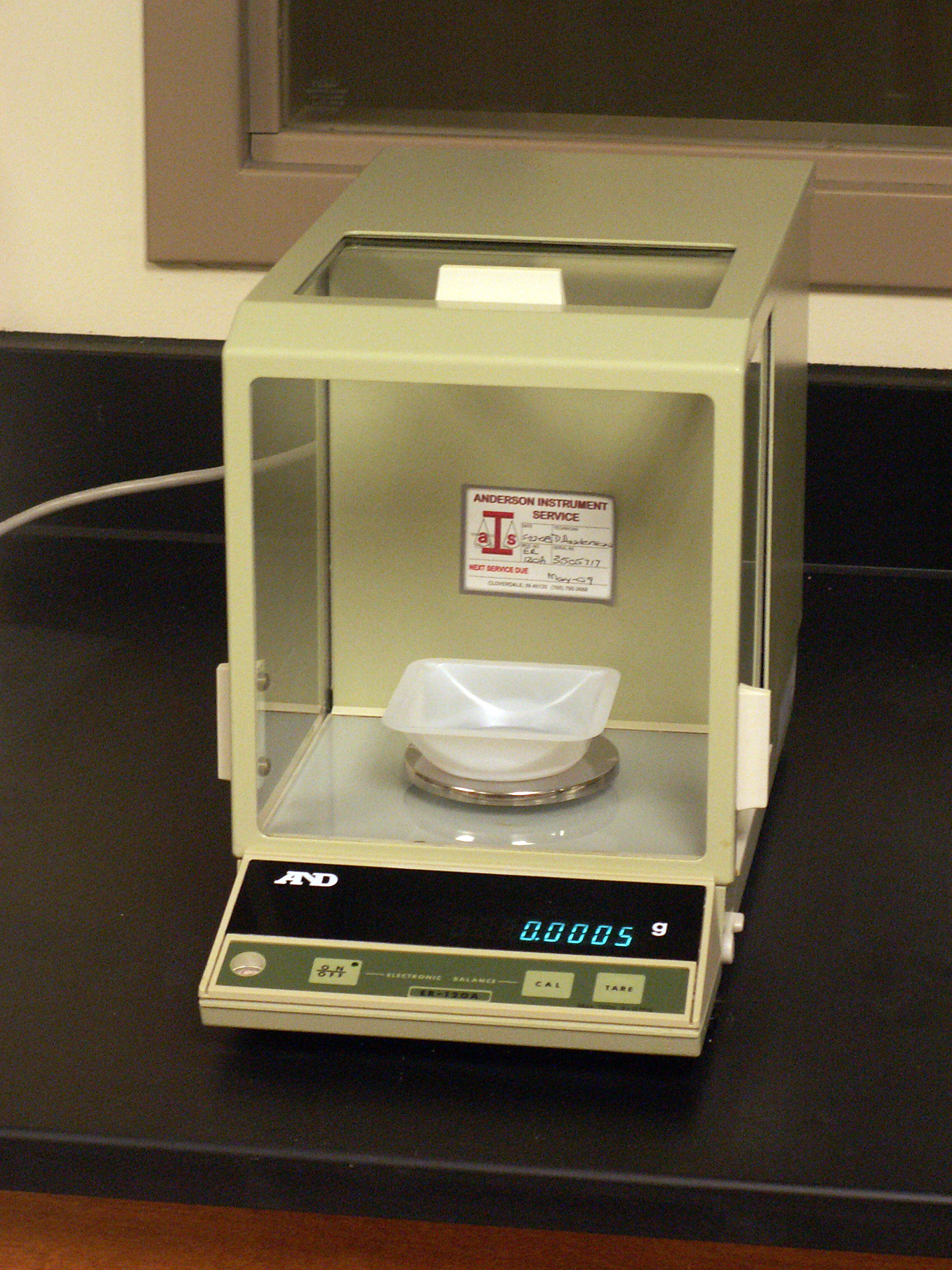
Although my doctor's balance beam scale encodes my mass by the position of two movable weights along a signal arm–a decidedly non-electrical means of encoding information—the electronic analytical balance that is found in almost all chemistry labs encodes the mass in the form of electrical information (Figure \(\PageIndex{1}\)). An electromagnet levitates the sample pan above a permanent cylindrical magnet. When we place an object on the sample pan, it displaces the sample pan downward by a force equal to the product of the sample’s mass and its acceleration due to gravity. The balance detects this downward movement and generates a counterbalancing force by increasing the current to the electromagnet. The current needed to return the balance to its original position is proportional to the object’s mass.
Although we tend to use interchangeably, the terms “weight” and “mass,” there is an important distinction between them. Mass is the absolute amount of matter in an object, measured in grams. Weight, W, is a measure of the gravitational force, g, acting on that mass, m:
\[W = m \times g \nonumber \]
An object has a fixed mass but its weight depends upon the acceleration due to gravity, which varies subtly from location-to-location.
A balance measures an object’s weight, not its mass. Because weight and mass are proportional to each other, we can calibrate a balance using a standard weight whose mass is traceable to the standard prototype for the kilogram. A properly calibrated balance gives an accurate value for an object’s mass.
Electrical information comes in three domains: analog, time, and digital. In the analog domain, the signal shows the amplitude of the electrical signal—say current or potential—as a function of an independent variable, which might be wavelength when recording a spectrum, applied potential in a cyclic voltammetry experiment, or time when separating a mixture by gas chromatography. A time domain signal shows the frequency with which the electrical signal rises above or below a threshold value, as when counting the rate at which ionizing radiation, such as alpha or beta particles, are detected by a Geiger counter. Finally, in the digital domain, the signal is a count of discrete events, such as counting the number of drops dispensed by an autotitrator by allowing the drops to disrupt a beam of light.
Input Transducers, Detectors, and Sensors
As defined above, a transducer is a device that converts information from a non-electrical form to an electrical form (the input transducer) or from an electrical form to a non-electrical form (the output transducer). Detector is a much broader term that includes all aspects of the instrument from the input transducer to the output transducer; thus, a visible spectrometer is a detector that uses an input transducer to convert the attenuation of the source radiation to a reported absorbance. A sensor is a detector designed to monitor a particular analyte, such as a pH electrode.
Output Transducers and Readout Devices
An instrument's output transducer converts the information carried in electrical form into a non-electrical form that we can understand. Common examples of output transducers, or readout devices, are a simple meter, a digital display, a physical trace of the signal as a function of a dependent variable, such as a spectrum or a chromatogram, or a photographic plate.
Computers in Instruments
Many instruments include a computer that provides us with the ability to control the instrument and, perhaps of greater importance, to process the data both by modifying the electrical signal as it passes from the input transducer to the output transducer, and by providing tools for processing the data after it leaves the output transducer.