
13.2: Chemical Kinetics
- Page ID
- 5587

\( \newcommand{\vecs}[1]{\overset { \scriptstyle \rightharpoonup} {\mathbf{#1}} } \)
\( \newcommand{\vecd}[1]{\overset{-\!-\!\rightharpoonup}{\vphantom{a}\smash {#1}}} \)
\( \newcommand{\id}{\mathrm{id}}\) \( \newcommand{\Span}{\mathrm{span}}\)
( \newcommand{\kernel}{\mathrm{null}\,}\) \( \newcommand{\range}{\mathrm{range}\,}\)
\( \newcommand{\RealPart}{\mathrm{Re}}\) \( \newcommand{\ImaginaryPart}{\mathrm{Im}}\)
\( \newcommand{\Argument}{\mathrm{Arg}}\) \( \newcommand{\norm}[1]{\| #1 \|}\)
\( \newcommand{\inner}[2]{\langle #1, #2 \rangle}\)
\( \newcommand{\Span}{\mathrm{span}}\)
\( \newcommand{\id}{\mathrm{id}}\)
\( \newcommand{\Span}{\mathrm{span}}\)
\( \newcommand{\kernel}{\mathrm{null}\,}\)
\( \newcommand{\range}{\mathrm{range}\,}\)
\( \newcommand{\RealPart}{\mathrm{Re}}\)
\( \newcommand{\ImaginaryPart}{\mathrm{Im}}\)
\( \newcommand{\Argument}{\mathrm{Arg}}\)
\( \newcommand{\norm}[1]{\| #1 \|}\)
\( \newcommand{\inner}[2]{\langle #1, #2 \rangle}\)
\( \newcommand{\Span}{\mathrm{span}}\) \( \newcommand{\AA}{\unicode[.8,0]{x212B}}\)
\( \newcommand{\vectorA}[1]{\vec{#1}} % arrow\)
\( \newcommand{\vectorAt}[1]{\vec{\text{#1}}} % arrow\)
\( \newcommand{\vectorB}[1]{\overset { \scriptstyle \rightharpoonup} {\mathbf{#1}} } \)
\( \newcommand{\vectorC}[1]{\textbf{#1}} \)
\( \newcommand{\vectorD}[1]{\overrightarrow{#1}} \)
\( \newcommand{\vectorDt}[1]{\overrightarrow{\text{#1}}} \)
\( \newcommand{\vectE}[1]{\overset{-\!-\!\rightharpoonup}{\vphantom{a}\smash{\mathbf {#1}}}} \)
\( \newcommand{\vecs}[1]{\overset { \scriptstyle \rightharpoonup} {\mathbf{#1}} } \)
\( \newcommand{\vecd}[1]{\overset{-\!-\!\rightharpoonup}{\vphantom{a}\smash {#1}}} \)
\(\newcommand{\avec}{\mathbf a}\) \(\newcommand{\bvec}{\mathbf b}\) \(\newcommand{\cvec}{\mathbf c}\) \(\newcommand{\dvec}{\mathbf d}\) \(\newcommand{\dtil}{\widetilde{\mathbf d}}\) \(\newcommand{\evec}{\mathbf e}\) \(\newcommand{\fvec}{\mathbf f}\) \(\newcommand{\nvec}{\mathbf n}\) \(\newcommand{\pvec}{\mathbf p}\) \(\newcommand{\qvec}{\mathbf q}\) \(\newcommand{\svec}{\mathbf s}\) \(\newcommand{\tvec}{\mathbf t}\) \(\newcommand{\uvec}{\mathbf u}\) \(\newcommand{\vvec}{\mathbf v}\) \(\newcommand{\wvec}{\mathbf w}\) \(\newcommand{\xvec}{\mathbf x}\) \(\newcommand{\yvec}{\mathbf y}\) \(\newcommand{\zvec}{\mathbf z}\) \(\newcommand{\rvec}{\mathbf r}\) \(\newcommand{\mvec}{\mathbf m}\) \(\newcommand{\zerovec}{\mathbf 0}\) \(\newcommand{\onevec}{\mathbf 1}\) \(\newcommand{\real}{\mathbb R}\) \(\newcommand{\twovec}[2]{\left[\begin{array}{r}#1 \\ #2 \end{array}\right]}\) \(\newcommand{\ctwovec}[2]{\left[\begin{array}{c}#1 \\ #2 \end{array}\right]}\) \(\newcommand{\threevec}[3]{\left[\begin{array}{r}#1 \\ #2 \\ #3 \end{array}\right]}\) \(\newcommand{\cthreevec}[3]{\left[\begin{array}{c}#1 \\ #2 \\ #3 \end{array}\right]}\) \(\newcommand{\fourvec}[4]{\left[\begin{array}{r}#1 \\ #2 \\ #3 \\ #4 \end{array}\right]}\) \(\newcommand{\cfourvec}[4]{\left[\begin{array}{c}#1 \\ #2 \\ #3 \\ #4 \end{array}\right]}\) \(\newcommand{\fivevec}[5]{\left[\begin{array}{r}#1 \\ #2 \\ #3 \\ #4 \\ #5 \\ \end{array}\right]}\) \(\newcommand{\cfivevec}[5]{\left[\begin{array}{c}#1 \\ #2 \\ #3 \\ #4 \\ #5 \\ \end{array}\right]}\) \(\newcommand{\mattwo}[4]{\left[\begin{array}{rr}#1 \amp #2 \\ #3 \amp #4 \\ \end{array}\right]}\) \(\newcommand{\laspan}[1]{\text{Span}\{#1\}}\) \(\newcommand{\bcal}{\cal B}\) \(\newcommand{\ccal}{\cal C}\) \(\newcommand{\scal}{\cal S}\) \(\newcommand{\wcal}{\cal W}\) \(\newcommand{\ecal}{\cal E}\) \(\newcommand{\coords}[2]{\left\{#1\right\}_{#2}}\) \(\newcommand{\gray}[1]{\color{gray}{#1}}\) \(\newcommand{\lgray}[1]{\color{lightgray}{#1}}\) \(\newcommand{\rank}{\operatorname{rank}}\) \(\newcommand{\row}{\text{Row}}\) \(\newcommand{\col}{\text{Col}}\) \(\renewcommand{\row}{\text{Row}}\) \(\newcommand{\nul}{\text{Nul}}\) \(\newcommand{\var}{\text{Var}}\) \(\newcommand{\corr}{\text{corr}}\) \(\newcommand{\len}[1]{\left|#1\right|}\) \(\newcommand{\bbar}{\overline{\bvec}}\) \(\newcommand{\bhat}{\widehat{\bvec}}\) \(\newcommand{\bperp}{\bvec^\perp}\) \(\newcommand{\xhat}{\widehat{\xvec}}\) \(\newcommand{\vhat}{\widehat{\vvec}}\) \(\newcommand{\uhat}{\widehat{\uvec}}\) \(\newcommand{\what}{\widehat{\wvec}}\) \(\newcommand{\Sighat}{\widehat{\Sigma}}\) \(\newcommand{\lt}{<}\) \(\newcommand{\gt}{>}\) \(\newcommand{\amp}{&}\) \(\definecolor{fillinmathshade}{gray}{0.9}\)The earliest analytical methods based on chemical kinetics—which first appear in the late nineteenth century—took advantage of the catalytic activity of enzymes. In a typical method of that era, an enzyme was added to a solution containing a suitable substrate and their reaction monitored for a fixed time. The enzyme’s activity was determined by the change in the substrate’s concentration. Enzymes also were used for the quantitative analysis of hydrogen peroxide and carbohydrates. The development of chemical kinetic methods continued in the first half of the twentieth century with the introduction of nonenzymatic catalysts and noncatalytic reactions.
Despite the diversity of chemical kinetic methods, by 1960 they were no longer in common use. The principal limitation to their broader acceptance was a susceptibility to significant errors from uncontrolled or poorly controlled variables—temperature and pH are two examples—and the presence of interferents that activate or inhibit catalytic reactions. By the 1980s, improvements in instrumentation and data analysis methods compensated for these limitations, ensuring the further development of chemical kinetic methods of analysis.3
13.2.1 Theory and Practice
Every chemical reaction occurs at a finite rate, making it a potential candidate for a chemical kinetic method of analysis. To be effective, however, the chemical reaction must meet three necessary conditions: the reaction must not occur too quickly or too slowly; we must know the reaction’s rate law; and we must be able to monitor the change in concentration for at least one species. Let’s take a closer look at each of these needs.
The material in this section assumes some familiarity with chemical kinetics, which is part of most courses in general chemistry. For a review of reaction rates, rate laws, and integrated rate laws, see the material in Appendix 17.
Reaction Rate
The rate of the chemical reaction—how quickly the concentrations of reactants and products change during the reaction—must be fast enough that we can complete the analysis in a reasonable time, but also slow enough that the reaction does not reach equilibrium while the reagents are mixing. As a practical limit, it is not easy to study a reaction that reaches equilibrium within several seconds without the aid of special equipment for rapidly mixing the reactants. We will discuss two examples of instrumentation for studying reactions with fast kinetics in Section 13.2.3.
Rate Law
The second requirement is that we must know the reaction’s rate law—the mathematical equation describing how the concentrations of reagents affect the rate—for the period in which we are making measurements. For example, the rate law for a reaction that is first order in the concentration of an analyte, A, is
\[ \mathrm{rate} = −\dfrac{ d[\ce A]}{dt} = k[\ce A] \label{13.1}\]
where k is the reaction’s rate constant.
Because the concentration of A decreases during the reactions, d[A] is negative. The minus sign in Equation \(\ref{13.1}\) makes the rate positive. If we choose to follow a product, P, then d[P] is positive because the product’s concentration increases throughout the reaction. In this case we omit the minus sign; see Equation \(\ref{13.21}\) for an example.
An integrated rate law often is a more useful form of the rate law because it is a function of the analyte’s initial concentration. For example, the integrated rate law for Equation \(\ref{13.1}\) is
\[ \ln[\ce A]_t = \ln[\ce A]_0 − kt \label{13.2}\]
or
\[[\ce A]_t = [\ce A]_0e^{−kt} \label{13.3}\]
where \([\ce A]_0\) is the analyte’s initial concentration and \([\ce A]_t\) is the analyte’s concentration at time \(t\).
Unfortunately, most reactions of analytical interest do not follow a simple rate law. Consider, for example, the following reaction between an analyte, A, and a reagent, R, to form a single product, \(\ce P\)
\[ \mathrm{A + R \underset{\mathit{k}_b}{\overset{\mathit{k}_f}{\rightleftharpoons}}P} \]
where \(k_\ce{f}\) is the rate constant for the forward reaction, and \(k_\ce{b}\) is the rate constant for the reverse reaction. If the forward and reverse reactions occur as single steps, then the rate law is
\[ \mathrm{rate = −\dfrac{\mathit{d}[A]}{\mathit{dt}} = \mathit{k}_f [A] [R] − \mathit{k}_b[P]} \label{13.4}\]
The first term of Equation \(\ref{13.4}\), \(k_\ce{f}\mathrm{[A][R]}\) accounts for the loss of \(\ce A\) as it reacts with \(\ce R\) to make \(\ce P\), and the second term, \(k_\ce{b}\mathrm{[P]}\) accounts for the formation of \(\ce A\) as \(\ce P\) converts back to \(\ce A\) and \(\ce R\).
Although we know the reaction’s rate law, there is no simple integrated form that we can use to determine the analyte’s initial concentration. We can simplify Equation \(\ref{13.4}\) by restricting our measurements to the beginning of the reaction when the product’s concentration is negligible. Under these conditions we can ignore the second term in Equation \(\ref{13.4}\), which simplifies to
\[ \mathrm{rate = - \dfrac{\mathit{d}[A]}{\mathit{dt}} = \mathit{k}_f[A] [R]} \label{13.5}\]
The integrated rate law for Equation \(\ref{13.5}\), however, is still too complicated to be analytically useful. We can further simplify the kinetics by carefully adjusting the reaction conditions.4 For example, we can ensure pseudo-first-order kinetics by using a large excess of R so that its concentration remains essentially constant during the time we are monitoring the reaction. Under these conditions Equation \(\ref{13.5}\) simplifies to
\[ \mathrm{rate = − \dfrac{\mathit{d}[A]}{\mathit{dt}} = \mathit{k}_f [A] [R]_0 = \mathit{k}′[A]} \label{13.6}\]
where \(k′ = k_\ce{f}[\ce R]_0\).
To say that the reaction is pseudo-first-order in A means that the reaction behaves as if it is first order in A and zero order in R even though the underlying kinetics are more complicated. We call \(k′\) the pseudo-first-order rate constant.
The integrated rate laws for Equation \(\ref{13.6}\) are
\[ \ln[\ce A]_t = \ln[\ce A]_0 − k′t \label{13.7}\]
or
\[ [\ce A]_t = [\ce A]_0e^{−k′t} \label{13.8}\]
It may even be possible to adjust the conditions so that we use the reaction under pseudo-zero-order conditions.
\[ \textrm{rate} = −\dfrac{d[\ce A]}{dt} = k_\ce{f}\mathrm{[A]_0[R]_0} = k′′ \label{13.9}\]
\[ [\ce A]_t = [\ce A]_0 − k′′t \label{13.10}\]
where \(k′′ = k_\ce{f} \mathrm{[A]_0[R]_0}\).
To say that a reaction is pseudo-zero-order means that the reaction behaves as if it is zero order in A and zero order in R even though the underlying kinetics are more complicated. We call \(k′′\) the pseudo-zero-order rate constant.
Equation \(\ref{13.10}\) is the integrated rate law for Equation \(\ref{13.9}\).
Monitoring the Reaction
The final requirement is that we must be able to monitor the reaction's progress by following the change in concentration for at least one of its species. Which species we choose to monitor is not important. It can be the analyte, a reagent reacting with the analyte, or a product. For example, we can determine concentration of phosphate in a sample by first reacting it with Mo(VI) to form 12.molybdophosphoric acid (12-MPA).
\[ \ce{H_3PO}_{4(aq)} + \ce{6Mo(VI)}_{(aq)}^+ → \textrm{12-MPA}_{(aq)} + \ce{9H^+}_{(aq)} \label{13.11}\]
Next, we reduce \(\textrm{12-MPA}\) to form heteropolyphosphomolybdenum blue, \(\textrm{PMB}\). The rate of formation of PMB is measured spectrophotometrically, and is proportional to the concentration of 12-MPA. The concentration of 12-MPA, in turn, is proportional to the concentration of phosphate.5 We also can follow reaction 13.11 spectrophotometrically by monitoring the formation of the yellow-colored 12-MPA.6
13.2.2 Classifying Chemical Kinetic Methods
Figure 13.2 provides one useful scheme for classifying chemical kinetic methods of analysis. Methods are divided into two main categories: direct-computation methods and curve-fitting methods. In a direct-computation method we calculate the analyte’s initial concentration, [A]0, using the appropriate rate law. For example, if the reaction is first-order in analyte, we can use Equation \(\ref{13.2}\) to determine [A]0 if we have values for k, t, and [A]t. With a curve-fitting method, we use regression to find the best fit between the data—for example, [A]t as a function of time—and the known mathematical model for the rate law. If the reaction is first-order in analyte, then we fit Equation \(\ref{13.2}\) to the data using k and [A]0 as adjustable parameters.
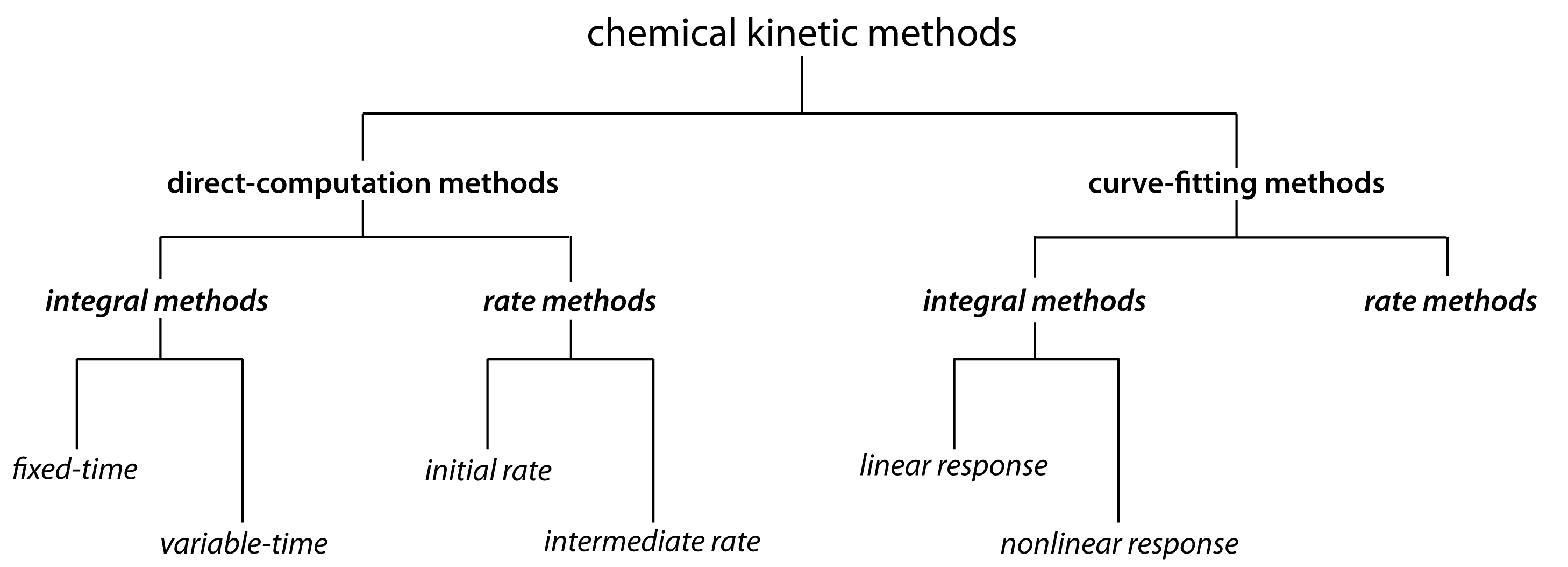
Figure 13.2: Classification of chemical kinetic methods of analysis adapted from Pardue, H. L. “Kinetic Aspects of Analytical Chemistry,” Anal. Chim. Acta 1989, 216, 69–107.
Direct-Computation Fixed-Time Integral Methods
A direct-computation integral method uses the integrated form of the rate law. In a one-point fixed-time integral method, for example, we determine the analyte’s concentration at a single time and calculate the analyte’s initial concentration, [A]0, using the appropriate integrated rate law. To determine the reaction’s rate constant, k, we run a separate experiment using a standard solution of analyte. Alternatively, we can determine the analyte’s initial concentration by measuring [A]t for several standards containing known concentrations of analyte and constructing a calibration curve.
Example 13.1
The concentration of nitromethane, CH3NO2, can be determined from the kinetics of its decomposition reaction. In the presence of excess base the reaction is pseudo-first-order in nitromethane. For a standard solution of 0.0100 M nitromethane, the concentration of nitromethane after 2.00 s is 4.24 × 10⁻⁴ M. When a sample containing an unknown amount of nitromethane is analyzed, the concentration of nitromethane remaining after 2.00 s is 5.35 × 10⁻⁴ M. What is the initial concentration of nitromethane in the sample?
Solution
First, we determine the value for the pseudo-first-order rate constant, k′. Using Equation \(\ref{13.7}\) and the result for the standard, we find its value is
\[k′ = \dfrac{\ln[\ce A]_0 − \ln[\ce A]_t}{t} = \mathrm{\dfrac{\ln(0.0100) − \ln(4.24×10^{−4})}{2.00\: s} = 1.58\: s^{−1}}\]
Next we use Equation \(\ref{13.8}\) to calculate the initial concentration of nitromethane in the sample.
\[\mathrm{[A]_0 = \dfrac{[A]_\mathit{t}}{\mathit{e^{−k^′t}}} = \dfrac{5.34×10^{−4}\: M}{\mathit{e}^{−(1.58\: s^{−1})(2.00\: s)}} = 0.0126\: M}\]
Note: Equation \(\ref{13.7}\) and Equation \(\ref{13.8}\) are equally appropriate integrated rate laws for a pseudo-first-order reaction. The decision to use Equation \(\ref{13.7}\) to calculate k′ and Equation \(\ref{13.8}\) to calculate [A]0 is a matter of convenience.
Exercise 13.1
In a separate determination for nitromethane, a series of external standards gives the following concentrations of nitromethane after a 2.00 s decomposition under pseudo-first-order conditions.
| [CH3NO2]0 (M) | [CH3NO2] (M) at t = 2.00 s |
|---|---|
| 0.0100 | 3.82×10⁻⁴ |
| 0.0200 | 8.19×10⁻⁴ |
| 0.0300 | 1.15×10⁻³ |
| 0.0400 | 1.65×10⁻³ |
| 0.0500 | 2.14×10⁻³ |
| 0.0600 | 2.53×10⁻³ |
| 0.0700 | 3.21×10⁻³ |
| 0.0800 | 3.35×10⁻³ |
| 0.0900 | 3.99×10⁻³ |
| 0.100 | 4.15×10⁻³ |
Analysis of a sample under the same conditions gives a nitromethane concentration of 2.21 × 10⁻³ M after 2 s. What is the initial concentration of nitromethane in the sample?
Click here to review your answer to this exercise.
In Example 13.1 we determined the initial concentration of analyte by measuring the amount of unreacted analyte. Sometimes it is more convenient to measure the concentration of a reagent that reacts with the analyte, or to measure the concentration of one of the reaction’s products. We can still use a one-point fixed-time integral method if we know the reaction’s stoichiometry. For example, if we measure the concentration of the product, P, in the reaction
\[\mathrm{A + R → P}\]
then the concentration of the analyte at time t is
\[[\ce A]_t = [\ce A]_0 - [\ce P]_t \label{13.12}\]
because the stoichiometry between the analyte and product is 1:1. If the reaction is pseudo-first-order in A, then substituting equation \(\ref{13.12}\) into equation \(\ref{13.7}\) gives
\[\ln([\ce A]_0 − [\ce P]_t) = \ln[\ce A]_0 − k′t \label{13.13}\]
which we simplify by writing in exponential form.
\[[\ce A]_0 - [\ce P]_t = [\ce A]_0e^{-k′t} \label{13.14}\]
Finally, solving equation \(\ref{13.14}\) for [A]0 gives the following equation.
\[[\ce A]_0 = \dfrac{[\ce P]_t}{1-e^{−k′t}} \label{13.15}\]
The kinetic method for phosphate described earlier is an example of a method in which we monitor the product. Because the phosphate ion does not absorb visible light, we incorporate it into a reaction that produces a colored product. That product, in turn, is converted into a different product that is even more strongly absorbing.
Example 13.2
The concentration of thiocyanate, SCN–, can be determined from the pseudo-first-order kinetics of its reaction with excess Fe3+ to form a reddish colored complex of Fe(SCN)2+. The reaction’s progress is monitored by measuring the absorbance of Fe(SCN)2+ at a wavelength of 480 nm. When using a standard solution of 0.100 M SCN–, the concentration of Fe(SCN)2+ after 10 s is 0.0516 M. The concentration of Fe(SCN)2+ in a sample containing an unknown amount of SCN– is 0.0420 M after 10 s. What is the initial concentration of SCN– in the sample?
Figure 6.15 shows the color of a solution containing the Fe(SCN)2+ complex.
Solution
First, we must determine a value for the pseudo-first-order rate constant, k′. Using equation \(\ref{13.13}\), we find that its value is
\[k′ = \mathrm{\dfrac{\ln[A]_0 − \ln([A]_0 − [P]_\mathit{t})}{\mathit{t}} = \dfrac{\ln(0.100) − \ln(0.100 − 0.0516)}{10.0\: s} = 0.0726\: s^{−1}}\]
Next, we use equation 13.15 to determine the initial concentration of SCN– in the sample.
\[\mathrm{[A]_0 = \dfrac{[P]_\mathit{t}}{1 − \mathit{e^{−k^′t}}} = \dfrac{0.0420\: M}{1 − \mathit{e}^{−(0.0726\: s^{−1})(10.0\: s)}} = 0.0814\: M}\]
Exercise 13.2
In a separate determination for SCN–, a series of external standards gives the following concentrations of Fe(SCN)2+ after a 10.0 s reaction with excess Fe3+ under pseudo-first-order conditions.
| [SCN−]0 (M) | [Fe(SCN)2+] (M) at t = 10.0 s |
|---|---|
| 5.00×10⁻³ | 1.79×10⁻³ |
| 1.50×10⁻² | 8.24×10⁻³ |
| 2.50×10⁻² | 1.28×10⁻² |
| 3.50×10⁻² | 1.85×10⁻² |
| 4.50×10⁻² | 2.21×10⁻² |
| 5.50×10⁻² | 2.81×10⁻² |
| 6.50×10⁻² | 3.27×10⁻² |
| 7.50×10⁻² | 3.91×10⁻² |
| 8.50×10⁻² | 4.34×10⁻² |
| 9.50×10⁻² | 4.89×10⁻² |
Analysis of a sample under the same conditions gives a Fe(SCN)2+ concentration of 3.52 × 10⁻² M after 10 s. What is the initial concentration of SCN– in the sample?
Click here to review your answer to this exercise.
A one-point fixed-time integral method has the advantage of simplicity because we need only a single measurement to determine the analyte’s initial concentration. As with any method that relies on a single determination, a one-point fixed-time integral method can not compensate for a constant determinate error. In a two-point fixed-time integral method we correct for constant determinate errors by making measurements at two points in time and using the difference between the measurements to determine the analyte’s initial concentration. Because it affects both measurements equally, the difference between the measurements is independent of a constant determinate error.
See Chapter 4 for a review of constant determinate errors and how they differ from proportional determinate errors.
For a pseudo-first-order reaction in which we measure the analyte’s concentration at times t1 and t2, we can write the following two equations.
\[ [\ce A]_{t_1} = [\ce A]_0e^{−k′t_1} \label{13.16}\]
\[ [\ce A]_{t_2} = [\ce A]_0e^{−k′t_2} \label{13.17}\]
Subtracting Equation \(\ref{13.17}\) from Equation \(\ref{13.16}\) and solving for \([A]_0\) leaves us with
\[ [\ce A]_0 = \dfrac{[\ce A]_{t_1} − [\ce A]_{t_2}}{e^{−k′t_1} − e^{−k′t_2}} \label{13.18}\]
To determine the rate constant, k′, we measure [A]t1 and [A]t2 for a standard solution of analyte. Having obtained a value for k′, we can determine [A]0 by measuring the analyte's concentration at t1 and t2. We can also determine the analyte's initial concentration using a calibration curve consisting of a plot of ([A]t1 – [A]t2) versus [A]0.
A fixed-time integral method is particularly useful when the signal is a linear function of concentration because we can replace the reactant’s concentration terms with the corresponding signal. For example, if we follow a reaction spectrophotometrically under conditions where the analyte’s concentration obeys Beer’s law
\[(Abs)_t = εb[\ce A]_t\]
then we can rewrite equation \(\ref{13.8}\) and equation \(\ref{13.18}\) as
\[(Abs)_t = [\ce A]_0e^{−k′t}εb=c[\ce A]_0\]
\[[\ce A]_0 = \dfrac{(Abs)_{t_1} − (Abs)_{t_2}}{e^{−k′t_1} −e^{−k′t_2}} × (εb)^{−1} =c′[(Abs)_{t_1} − (Abs)_{t_2}]\]
where (Abs)t is the absorbance at time t, and c and c′ are constants.
Note
\[c = e^{−k′t}εb\]
\[c′ = \dfrac{1}{(εb)\left(e^{−k′t_1} − e^{−k′t_2}\right)}\]
Direct-Computation Variable-Time Integral Methods
In a variable-time integral method we measure the total time, ∆t, needed to effect a specific change in concentration for one species in the chemical reaction. One important application is for the quantitative analysis of catalysts, which takes advantage of the catalyst’s ability to increase the rate of reaction. As the concentration of catalyst increase, ∆t decreases. For many catalytic systems the relationship between ∆t and the catalyst’s concentration is
\[ \dfrac{1}{∆t} =F_\ce{cat}[A]_0 + F_\ce{uncat} \label{13.19}\]
where [A]0 is the catalyst’s concentration, and \(F_\ce{cat}\) and \(F_\ce{uncat}\) are constants accounting for the rate of the catalyzed and uncatalyzed reactions.7
Example 13.3
Sandell and Kolthoff developed a quantitative method for iodide based on its ability to catalyze the following redox reaction.8
\[\ce{As^3+}(aq) + \ce{2Ce^4+}(aq) → \ce{As^5+}(aq) + \ce{2Ce^3+}(aq)\]
An external standards calibration curve was prepared by adding 1 mL of a KI standard to a mixture consisting of 2 mL of 0.05 M As3+, 1 mL of 0.1 M Ce4+, and 1 mL of 3 M H2SO4, and measuring the time for the yellow color of Ce4+ to disappear. The following table summarizes the results for one analysis.
| [I−] (μg/mL) | ∆t (min) |
|---|---|
| 5.0 | 0.9 |
| 2.5 | 1.8 |
| 1.0 | 4.5 |
What is the concentration of I– in a sample ∆t is 3.2 min?
Solution
Figure 13.3 shows the calibration curve and calibration equation for the external standards based on equation 13.19. Substituting 3.2 min for ∆t gives the concentration of I– in the sample as 1.4 μg/mL.

Figure 13.3 Calibration curve and calibration equation for Example 13.3.
Direct-Computation Rate Methods
In a rate method we use the differential form of the rate law—Equation \(\ref{13.1}\) is one example of a differential rate law—to determine the analyte’s concentration. As shown in Figure 13.4, the rate of a reaction at time \(t\), \((rate)_t\), is the slope of a line tangent to a curve showing the change in concentration as a function of time. For a reaction that is first-order in analyte, the rate at time \(t\) is
\[(\ce{rate})_t = k[\ce A]_t\]
Substituting in Equation \(\ref{13.3}\) leaves us with the following equation relating the rate at time t to the analyte’s initial concentration.
\[(\ce{rate})_t = k[\ce A]_0e^{−kt}\]
If we measure the rate at a fixed time, then both \(k\) and \(e^{–kt}\) are constant and we can use a calibration curve of (rate)t versus [A]0 for the quantitative analysis of the analyte.
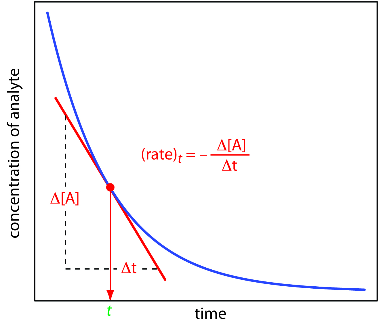
Figure 13.4: Determination of a reaction’s intermediate rate from the slope of a line tangent to a curve showing the change in the analyte’s concentration as a function of time.
There are several advantages to using the reaction’s initial rate (t = 0). First, because the reaction’s rate decreases over time, the initial rate provides the greatest sensitivity. Second, because the initial rate is measured under nearly pseudo-zero-order conditions, in which the change in concentration with time is effectively linear, the determination of slope is easier. Finally, as the reaction of interest progresses competing reactions may develop, complicating the kinetics—using the initial rate eliminates these complications. One disadvantage of the initial rate method is that there may be insufficient time for completely mixing the reactants. This problem is avoided by using an intermediate rate measured at a later time (t > 0).
As a general rule (see Mottola, H. A. “Kinetic Determinations of Reactants Utilizing Uncatalyzed Reactions,” Anal. Chim. Acta 1993, 280, 279–287), the time for measuring a reaction’s initial rate should result in the consumption of no more than 2% of the reactants. The smaller this percentage, the more linear the change in concentration as a function of time.
Example 13.4
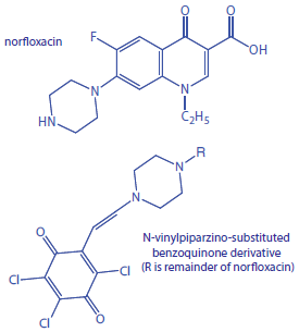
The concentration of norfloxacin, a commonly prescribed antibacterial agent, is determined using the initial rate method. Norfloxacin is converted to an N-vinylpiperazine derivative and reacted with 2,3,5,6-tetrachloro-1,4-benzoquinone to form an N-vinylpiperazino-substituted benzoquinone derivative that absorbs strongly at 625 nm.9 The initial rate of the reaction—as measured by the change in absorbance as a function of time (AU/min)—is pseudo-first order in norfloxacin. The following data were obtained for a series of external norfloxacin standards.
| [norfloxacin] (μg/mL) | initial rate (AU/min) |
|---|---|
| 63 | 0.0139 |
| 125 | 0.0355 |
| 188 | 0.0491 |
| 251 | 0.0656 |
| 313 | 0.0859 |
To analyze a sample of prescription eye drops, a 10.00-mL portion was extracted with dichloromethane. The extract was dried and the norfloxacin reconstituted in methanol and diluted to 10 mL in a volumetric flask. A 5.00-mL portion of this solution was diluted to volume in a 100-mL volumetric flask. Analysis of this sample gave an initial rate of 0.0394 AU/min. What is the concentration of norfloxacin in the eye drops? AU stands for absorbance unit.
Solution
Figure 13.5 shows the calibration curve and calibration equation for the external standards. Substituting 0.0394 AU/min for the initial rate and solving for the concentration of norfloxacin gives a result of 152 mg/mL. This is the concentration in a diluted sample of the extract. The concentration in the extract before dilution is
\[\mathrm{\dfrac{152\: g}{mL} × \dfrac{100.0\: mL}{5.00\: mL} × \dfrac{1\: g}{1000\: mg} = 3.04\: mg/mL}\]
Because the dried extract was reconstituted using a volume identical to that of the original sample, the concentration of norfloxacin in the eye drops is 3.04 mg/mL.
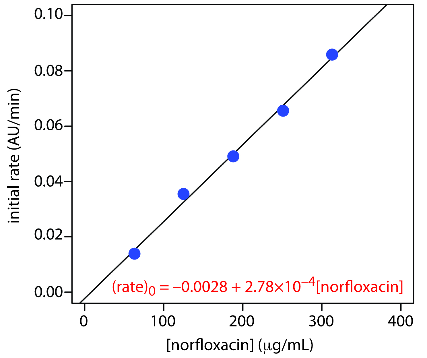
Figure 13.5: Calibration curve and calibration equation for Example 13.4.
Curve-Fitting Methods
In direct-computation methods we determine the analyte’s concentration by solving the appropriate rate equation at one or two discrete times. The relationship between the analyte’s concentration and the measured response is a function of the rate constant, which we determine in a separate experiment using a single external standard (see Example 13.1 or Example 13.2), or a calibration curve (see Example 13.3 or Example 13.4).
In a curve-fitting method we continuously monitor the concentration of a reactant or a product as a function of time and use a regression analysis to fit the data to an appropriate differential rate law or integrated rate law. For example, if we are monitoring the concentration of a product for a reaction that is pseudo-first-order in the analyte, then we can fit the data to the following rearranged form of Equation \(\ref{13.15}\)
\[[\ce P]_t = [\ce A]_0(1 − e^{−k′t})\]
using [A]0 and k′ as adjustable parameters. Because we are using data from more than one or two discrete times, a curve-fitting method is capable of producing more reliable results.
Example 13.5
The data shown in the following table were collected for a reaction that is known to be pseudo-zero-order in analyte.
| time (s) | [A]t (mM) | time (s) | [A]t (mM) |
|---|---|---|---|
| 3 | 0.0731 | 8 | 0.0448 |
| 4 | 0.0728 | 9 | 0.0404 |
| 5 | 0.0681 | 10 | 0.0339 |
| 6 | 0.0582 | 11 | 0.0217 |
| 7 | 0.0511 | 12 | 0.0143 |
What is the initial concentration of analyte in the sample and the rate constant for the reaction?
Solution
From equation 13.10 we know that for a pseudo-zero-order reaction a plot of [A]t versus time is linear with a slope of –k″, and a y-intercept of [A]0. Figure 13.6 shows a plot of the kinetic data and the result of a linear regression analysis. The initial concentration of analyte is 0.0986 mM and the rate constant is 0.00677 M–1 s–1.
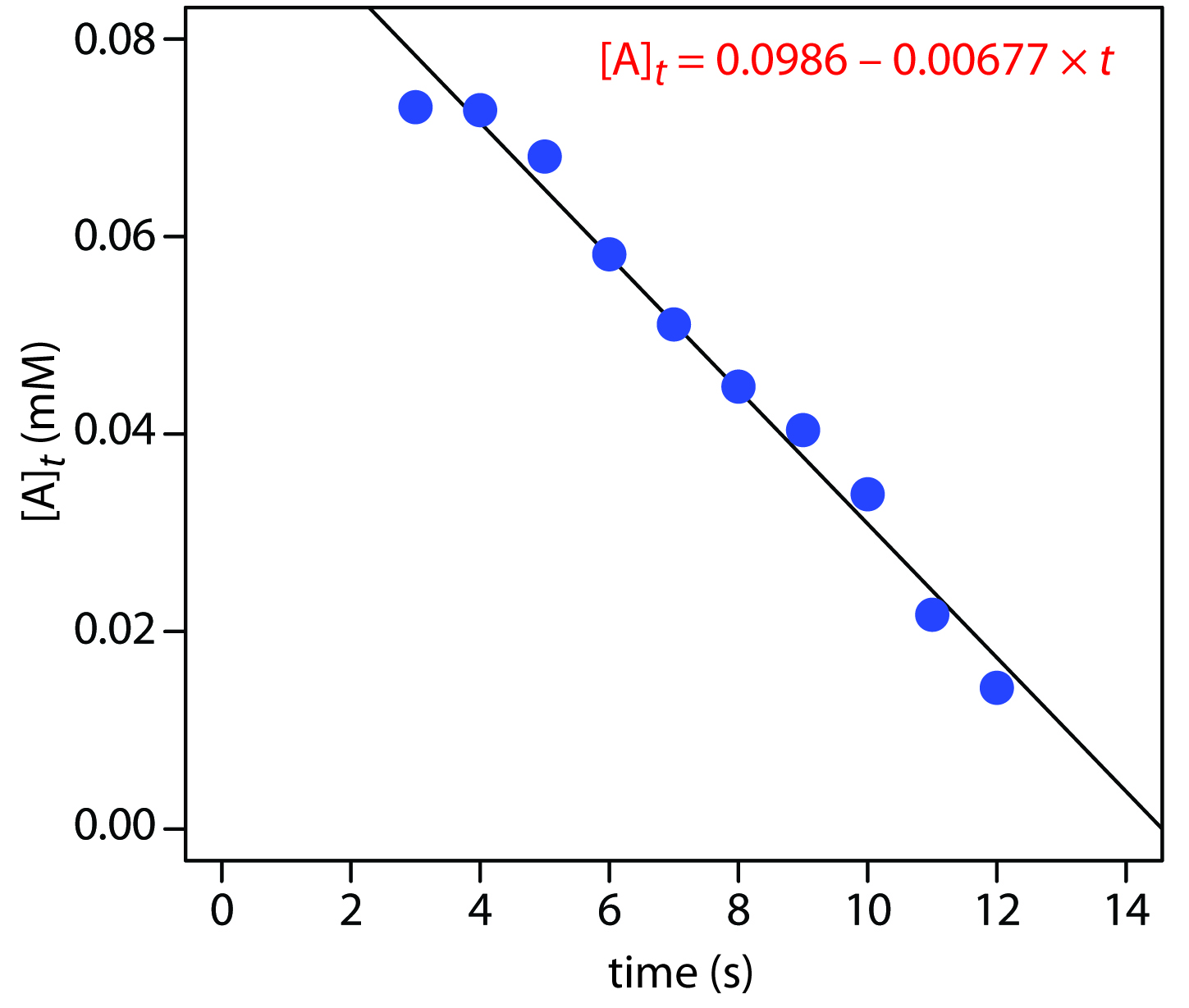
Figure 13.6 Result of fitting equation 13.10 to the data in Example 13.5.
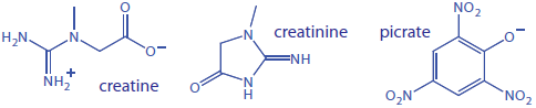
The best way to appreciate the theoretical and practical details discussed in this section is to carefully examine a typical analytical method. Although each method is unique, the following description of the determination of creatinine in urine provides an instructive example of a typical procedure. The description here is based on Diamandis, E. P.; Koupparis, M. A.; Hadjiioannou, T. P. “Kinetic Studies with Ion Selective Electrodes: Determination of Creatinine in Urine with a Picrate Ion Selective Electrode,” J. Chem. Educ. 1983, 60, 74–76.
Representative Method 13.1: Determination of Creatinine in Urine
Description of Method
Creatine is an organic acid found in muscle tissue that supplies energy for muscle contractions. One of its metabolic products is creatinine, which is excreted in urine. Because the concentration of creatinine in urine and serum is an important indication of renal function, rapid methods for its analysis are clinically important. In this method the rate of reaction between creatinine and picrate in an alkaline medium is used to determine the concentration of creatinine in urine. Under the conditions of the analysis the reaction is first order in picrate, creatinine, and hydroxide.
\[\mathrm{rate = \mathit{k} [picrate] [creatinine] [OH^−]}\]
The reaction is monitored using a picrate ion selective electrode.
Procedure
Prepare a set of external standards containing 0.5–3.0 g/L creatinine using a stock solution of 10.00 g/L creatinine in 5 mM H2SO4, diluting each to volume using 5 mM H2SO4. Prepare a solution of 1.00 × 10⁻² M sodium picrate. Pipet 25.00 mL of 0.20 M NaOH, adjusted to an ionic strength of 1.00 M using Na2SO4, into a thermostated reaction cell at 25oC. Add 0.500 mL of the 1.00 × 10⁻² M picrate solution to the reaction cell. Suspend a picrate ion selective in the solution and monitor the potential until it stabilizes. When the potential is stable, add 2.00 mL of a creatinine external standard and record the potential as a function of time. Repeat this procedure using the remaining external standards. Construct a calibration curve of ∆E/∆t versus the initial concentration of creatinine. Use the same procedure to analyze samples, using 2.00 mL of urine in place of the external standard. Determine the concentration of creatinine in the sample using the calibration curve.
Questions
1. The analysis is carried out under conditions that are pseudo-first order in picrate. Show that under these conditions the change in potential as a function of time is linear.
The potential, E, of the picrate ion selective electrode is given by the Nernst equation
\[E = K - \dfrac{RT}{F}\ln[\ce{picrate}]\]
where K is a constant that accounts for the reference electrodes, junction potentials, and the ion selective electrode’s asymmetry potential, R is the gas constant, T is the temperature, and F is Faraday’s constant.
(For a review of the Nernst equation for ion selective electrodes, see Section 11.2.3 in Chapter 11.)
We know from equation 13.7 that for a pseudo-first-order reaction, the concentration of picrate at time t is
\[\ln[\ce{picrate}]_t = \ln[\ce{picrate}]_0 - k′t\]
where k′ is the pseudo-first-order rate constant. Substituting this integrated rate law into the ion selective electrode’s Nernst equation leave us with the following result.
\[E_t = K - \dfrac{RT}{F}(\ln[\ce{picrate}]_0 − k′t)\]
\[E_t = K − \dfrac{RT}{F}\ln[\ce{picrate}]_0 + \dfrac{RT}{F}k′t\]
Because K and (RT/F)ln[picrate]0 are constants, a plot of Et versus t is a straight line with a slope of RTk′/F.
2. Under the conditions of the analysis the rate of the reaction is pseudo-first-order in picrate and pseudo-zero-order in creatinine and OH–. Explain why it is possible to prepare a calibration curve of ∆E/∆t versus the concentration of creatinine.
The slope of a plot of Et versus t is ∆E/∆t = RTk′/F (see the previous question). Because the reaction is carried out under conditions where it is pseudo-zero-order in creatinine and OH–, the rate law is
\[\ce{rate} = k\ce{[picrate] [creatinine]0[OH- ]0} = k′[\ce{picrate}]\]
The pseudo-first-order rate constant, k′, is
\[k′ = k\ce{[creatinine]0[OH- ]0} = c\ce{[creatinine]0}\]
\[\dfrac{E}{t} = \dfrac{RTk′}{F} =\dfrac{RTc}{F}\ce{[creatinine]0}\]
and a plot of ∆E/∆t versus the concentration of creatinine can serve as a calibration curve.
3. Why is it necessary to thermostat the reaction cell?
The rate of a reaction is temperature-dependent. To avoid a determinate error resulting from a systematic change in temperature, or to minimize indeterminate errors due to fluctuations in temperature, the reaction cell is thermostated to maintain a constant temperature.
4. Why is it necessary to prepare the NaOH solution so that it has an ionic strength of 1.00 M?
The potential of the picrate ion selective electrode actually responds to the activity of the picrate anion in solution. By adjusting the NaOH solution to a high ionic strength we maintain a constant ionic strength in all standards and samples. Because the relationship between activity and concentration is a function of ionic strength, the use of a constant ionic strength allows us to write the Nernst equation in terms of picrate’s concentration instead of its activity.
For a review of the relationship between concentration, activity, and ionic strength, see Chapter 6.9.
13.2.3 Making Kinetic Measurements
When using Representative Method 13.1 to determine the concentration of creatinine in urine, we follow the reactions kinetics using an ion selective electrode. In principle, we can use any of the analytical techniques in Chapters 8–12 to follow a reaction’s kinetics provided that the reaction does not proceed to any appreciable extent during the time it takes to make a measurement. As you might expect, this requirement places a serious limitation on kinetic methods of analysis. If the reaction’s kinetics are slow relative to the analysis time, then we can make our measurements without the analyte undergoing a significant change in concentration. When the reaction’s rate is too fast—which often is the case—then we introduce a significant error if our analysis time is too long.
One solution to this problem is to stop, or quench the reaction by adjusting experimental conditions. For example, many reactions show a strong pH dependency, and may be quenched by adding a strong acid or a strong base. Figure 13.7 shows a typical example for the enzymatic analysis of p-nitrophenylphosphate using the enzyme wheat germ acid phosphatase to hydrolyze the analyte to p-nitrophenol.
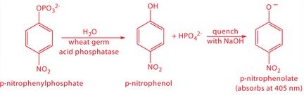
The reaction has a maximum rate at a pH of 5. Increasing the pH by adding NaOH quenches the reaction and converts the colorless p-nitrophenol to the yellow-colored p-nitrophenolate, which absorbs at 405 nm.
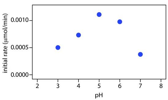
Figure 13.7: Initial rate for the enzymatic hydrolysis of p-nitrophenylphosphate using wheat germ acid phosphatase. Increasing the pH quenches the reaction and coverts colorless p-nitrophenol to the yellow-colored p-nitrophenolate, which absorbs at 405 nm. The data are adapted from socrates.hunter.cuny.edu.
An additional experimental problem when the reaction’s kinetics are fast is ensuring that we rapidly and reproducibly mix the sample and the reagents. For a fast reaction we need to make measurements in a few seconds, or even a few milliseconds. This presents us with both a problem and an important advantage. The problem is that rapidly and reproducibly mixing the sample and the reagent requires a dedicated instrument, which adds an additional expense to the analysis. The advantage is that a rapid, automated analysis allows for a high throughput of samples. Instrumentation for the automated kinetic analysis of phosphate using reaction 13.11, for example, have sampling rates of approximately 3000 determinations per hour.
A variety of instruments have been developed to automate the kinetic analysis of fast reactions. One example, which is shown in Figure 13.8, is the stopped-flow analyzer. The sample and reagents are loaded into separate syringes and precisely measured volumes are dispensed into a mixing chamber by the action of a syringe drive. The continued action of the syringe drive pushes the mixture through an observation cell and into a stopping syringe. The back pressure generated when the stopping syringe hits the stopping block completes the mixing, after which the reaction’s progress is monitored spectrophotometrically. With a stopped-flow analyzer it is possible to complete the mixing of sample and reagent, and initiate the kinetic measurements in approximately 0.5 ms. By attaching an autosampler to the sample syringe it is possible to analyze up to several hundred samples per hour.
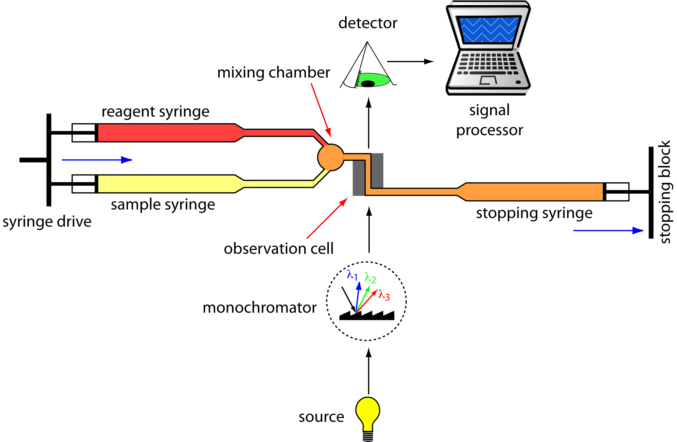
Figure 13.8: Schematic diagram of a stopped-flow analyzer. The blue arrows show the direction in which the syringes are moving.
Another instrumental design is the centrifugal analyzer, a partial cross section of which is shown in Figure 13.9. The sample and the reagents are placed in separate wells, which are oriented radially around a circular transfer disk. As the centrifuge spins, the centrifugal force pulls the sample and the reagents into the cuvette where mixing occurs. A single optical source and detector, located below and above the transfer disk’s outer edge, measures the absorbance each time the cuvette passes through the optical beam. When using a transfer disk with 30 cuvettes and rotating at 600 rpm, we can collect 10 data points per second for each sample.
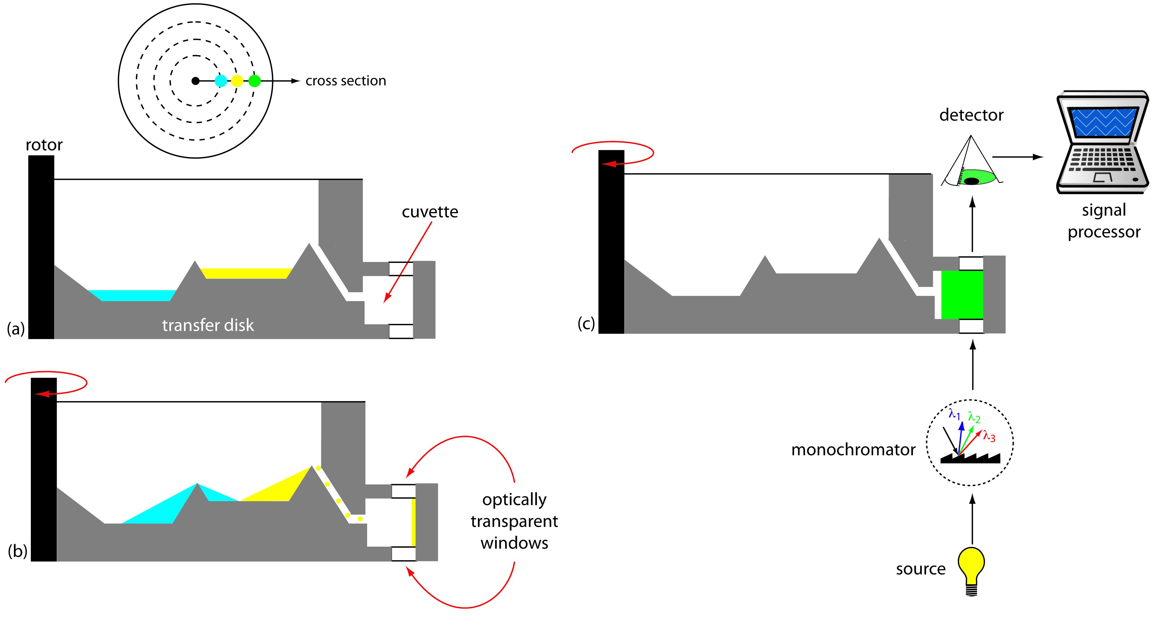
Figure 13.9: Cross sections through a centrifugal analyzer showing (a) the wells holding the sample and the reagents, (b) the mixing of the sample and the reagents, and (c) the configuration of the spectrophotometric detector.
The ability to collect lots of data and to collect it quickly requires appropriate hardware and software. Not surprisingly, automated kinetic analyzers developed in parallel with advances in analog and digital circuitry—the hardware—and computer software for smoothing, integrating, and differentiating the analytical signal. For an early discussion of the importance of hardware and software, see Malmstadt, H. V.; Delaney, C. J.; Cordos, E. A. “Instruments for Rate Determinations,” Anal. Chem. 1972, 44(12), 79A–89A.
13.2.4 Quantitative Applications
Chemical kinetic methods of analysis continue to find use for the analysis of a variety of analytes, most notably in clinical laboratories where automated methods aid in handling the large volume of samples. In this section we consider several general quantitative applications.
Enzyme-Catalyzed Reactions
Enzymes are highly specific catalysts for biochemical reactions, with each enzyme showing a selectivity for a single reactant, or substrate. For example, the enzyme acetylcholinesterase catalyzes the decomposition of the neurotransmitter acetylcholine to choline and acetic acid. Many enzyme–substrate reactions follow a simple mechanism that consists of the initial formation of an enzyme–substrate complex, \(ES\), which subsequently decomposes to form product, releasing the enzyme to react again.
\[ \mathrm{\large E + S \underset{\mathit{k}_{-1}}{\overset{\mathit{k}_1}{\rightleftharpoons}} ES \underset{\mathit{k}_{-2}}{\overset{\mathit{k}_2}{\rightleftharpoons}} E + P} \label{13.20}\]
where \(k_1\), \(k_{–1}\), \(k_2\), and \(k_{–2}\) are rate constants. If we make measurement early in the reaction, the concentration of products is negligible and we can ignore the step described by the rate constant \(k_{–2}\). Under these conditions the reaction’s rate is
\[ \ce{rate} = \dfrac{d[\ce P]}{dt} = k_2[\ce{ES}] \label{13.21}\]
To be analytically useful we need to write Equation \(\ref{13.21}\) in terms of the concentrations of enzyme and substrate. To do this we use the steady-state approximation, in which we assume that the concentration of \(ES\) remains essentially constant. Following an initial period, during which the enzyme–substrate complex first forms, the rate at which \(ES\) forms
\[ \dfrac{d[\ce{ES}]}{dt} =k_1\mathrm{[E] [S]} = k_1\mathrm{([E]_0 − [ES])[S]} \label{13.22}\]
is equal to the rate at which it disappears
\[ − \dfrac{d[\ce{ES}]}{dt} = k_{−1}[\ce{ES}] + k_2[\ce{ES}] \label{13.23}\]
where \([E]_0\) is the enzyme’s original concentration. Combining Equations \(\ref{13.22}\) and \(\ref{13.23}\) gives
\[k_1\mathrm{([E]_0 − [ES]) [S]} = k_{−1}[\ce{ES}] + k_2[\ce{ES}]\]
which we solve for the concentration of the enzyme–substrate complex
\[ [ES] = \dfrac{ \mathrm{[E]_0[S]} }{ \dfrac{k_{−1} + k_2}{k_1} + [S] } = \dfrac{\mathrm{[E]_0[S]} }{K_\ce{m} + [S]} \label{13.24}\]
where \(K_\ce{m}\) is the Michaelis constant. Substituting Equation \(\ref{13.24}\) into Equation \(\ref{13.21}\) leaves us with our final rate equation.
\[ \dfrac{d[\ce P]}{dt} = \dfrac{k_2\mathrm{[E]_0[S]}}{K_\ce{m} + [S]} \label {13.25} \]
A plot of Equation \(\ref{13.25}\), as shown in Figure 13.10, is instructive for defining conditions where we can use the rate of an enzymatic reaction for the quantitative analysis of an enzyme or substrate. For high substrate concentrations, where \([\ce S] >> K_\ce{m}\), Equation \(\ref{13.25}\) simplifies to
\[ \dfrac{d[\ce P]}{dt} = \dfrac{k_2\mathrm{[E]_0[S]}}{ K_\ce{m} + [S]} \approx \dfrac{k_2\mathrm{[E]_0[S]}}{[S]} = k_2[\ce E]_0 = V_\ce{max} \label{13.26}\]
where \(V_\ce{max}\) is the maximum rate for the catalyzed reaction. Under these conditions the reaction is pseudo-zero-order in substrate, and we can use \(V_\ce{max}\) to calculate the enzyme’s concentration, typically using a variable-time method. At lower substrate concentrations, where \([\ce S] << K_\ce{m}\), Equation \(\ref{13.25}\) becomes
\[ \dfrac{d[\ce P]}{dt} = \dfrac{k_2\mathrm{[E]_0[S]}}{K_\ce{m} + [S]} \approx \dfrac{k_2\mathrm{[E]_0[S]}}{ K_\ce{m}} =\dfrac{V_\ce{max}[\ce S]}{K_\ce{m}} \label{13.27}\]
The reaction is now first-order in substrate, and we can use the rate of the reaction to determine the substrate’s concentration by a fixed-time method.
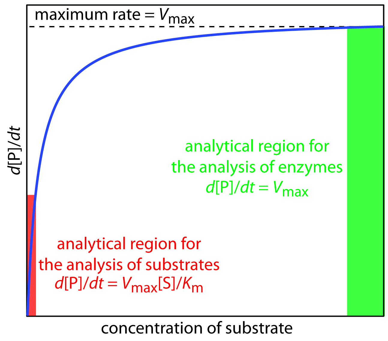
Figure 13.10: Plot of Equation \(\ref{13.25}\) showing limits for the analysis of substrates and enzymes in an enzyme-catalyzed chemical kinetic method of analysis. The curve in the region highlighted in red obeys Equation \(\ref{13.27}\) and the curve in the area highlighted in green follows Equation \(\ref{13.26}\).
Chemical kinetic methods have been applied to the quantitative analysis of a number of enzymes and substrates.10 One example, is the determination of glucose based on its oxidation by the enzyme glucose oxidase
\[\ce{glucose}_{(aq)} + \ce{H_2O}_{(l)} + \ce{O}_{2(aq)} \overset{\text{glucose oxidase}}{\rightarrow} \ce{gluconolactone}_{(aq)} + \ce{H_2O}_{2(aq)}\]
under conditions where Equation \(\ref{13.20}\) is valid. The reaction is monitored by following the rate of change in the concentration of dissolved \(\ce{O_2}\) using an appropriate voltammetric technique.
One method for measuring the concentration of dissolved O2 is the Clark amperometric sensor described in Chapter 11.
Nonenzyme-Catalyzed Reactions
The variable-time method has also been used to determine the concentration of nonenzymatic catalysts. One of the most commonly used reactions is the reduction of \(\ce{H_2O_2}\) by reducing agents such as thiosulfate, iodide, and hydroquinone. These reactions are catalyzed by trace amounts of selected metal ions. For example the reduction of \(\ce{H_2O_2}\) by \(\ce{I^-}\)
\[\ce{2I^-}_{(aq)} + \mathrm{H_2O}_{2(aq)} + \ce{2H_3O^+}_{(aq)} → \ce{4H2O}_{(l)} + \ce{I}_{2(aq)}\]
is catalyzed by \(\ce{Mo(VI)}\), \(\ce{W(VI)}\), and \(\ce{Zr(IV)}\). A variable-time analysis is conducted by adding a small, fixed amount of ascorbic acid to each solution. As \(\ce{I_2}\) is produced it rapidly oxidizes the ascorbic acid, and is reduced back to \(\ce{I^-}\). Once all the ascorbic acid is consumed, the presence of excess \(\ce{I_2}\) provides a visual endpoint.
Noncatalytic Reactions
Chemical kinetic methods are not as common for the quantitative analysis of analytes in noncatalytic reactions. Because they lack the enhancement of reaction rate that a catalyst affords, noncatalytic methods generally are not useful for determining small concentrations of analytes. Noncatalytic methods for inorganic analytes are usually based on a complexation reaction. One example is the determination of aluminum in serum by measuring the initial rate for the formation of its complex with 2-hydroxy-1-napthaldehyde p-methoxybenzoyl-hydrazone.11 The greatest number of noncatalytic methods, however, are for the quantitative analysis of organic analytes. For example, the insecticide methyl parathion has been determined by measuring its rate of hydrolysis in alkaline solutions.12
13.2.5 Characterization Applications
Chemical kinetic methods also find use in determining rate constants and in elucidating reaction mechanisms. Two examples from the kinetic analysis of enzymes illustrate these applications.
Determining Vmax and Km for Enzyme-Catalyzed Reactions
The value of Vmax and Km for an enzymatic reaction are of significant interest in the study of cellular chemistry. For an enzyme following the mechanism in reaction \(\ref{13.20}\), \(V_\ce{max}\) is equivalent to \(k_2[\ce E]_0\), where \([\ce E]_0\) is the enzyme’s concentration and \(k_2\) is the enzyme’s turnover number. The turnover number is the maximum number of substrate molecules converted to product by a single active site on the enzyme, per unit time. A turnover number, therefore, provides a direct indication of the active site’s catalytic efficiency. The Michaelis constant, \(K_\ce{m}\), is significant because it provides an estimate of the substrate’s intracellular concentration.13
Turnover Rate
An enzyme’s turnover number also is know as \(k_\ce{cat}\) and is equal to \(V_\ce{max}/[\ce E]_0\). For the mechanism in reaction \(\ref{13.20}\), \(k_\ce{cat}\) is equivalent to \(k_2\). For more complicated mechanisms, \(k_\ce{cat}\) is a function of additional rate constants.
As shown in Figure 13.10, we can find values for \(V_\ce{max}\) and \(K_\ce{m}\) by measuring the reaction’s rate for small and for large concentrations of the substrate. Unfortunately, this is not always practical as the substrate’s limited solubility may prevent us from using the large substrate concentrations needed to determine \(V_\ce{max}\). Another approach is to rewrite Equation \(\ref{13.25}\) by taking its reciprocal
\[ \dfrac{1}{d[\ce P] / dt} = \dfrac{1}{v} =\dfrac{K_\ce{m}}{V_\ce{max}} \times \dfrac{1}{[\ce S]} + \dfrac{1}{V_\ce{max}} \label{13.28}\]
where \(v\) is the reaction’s rate. As shown in Figure 13.11, a plot of \(\frac{1}{v}\) versus \(\frac{1}{[\ce S]}\), which is called a double reciprocal or Lineweaver–Burk plot, is a straight line with a slope of \(\frac{K_\ce{m}}{V_\ce{max}}\), a y-intercept of \(1/V_\ce{max}\), and an x-intercept of \(–\frac{1}{K_\ce{m}}\).
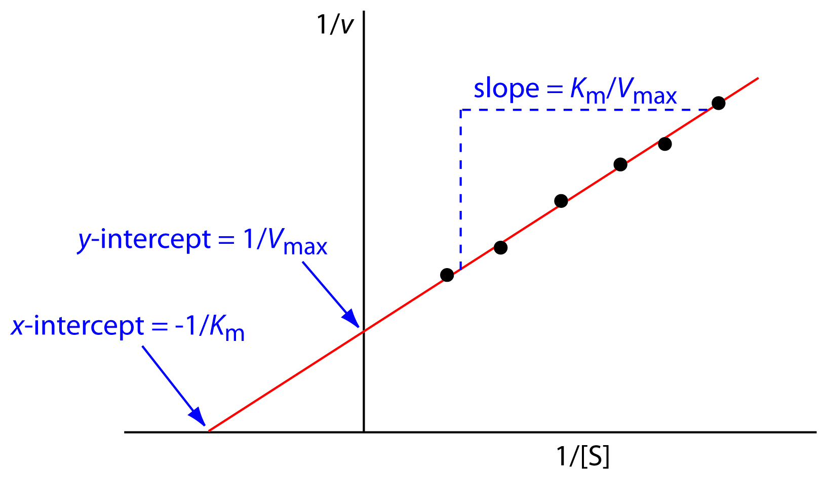
Figure 13.11: Lineweaver–Burk plot of Equation \(\ref{13.25}\) using Equation \(\ref{13.28}\).
In Chapter 5 we noted that when faced with a nonlinear model—and Equation \(\ref{13.25}\) is one example of a nonlinear model—it may be possible to rewrite the equation in a linear form. This is the strategy used here. Linearizing a nonlinear model is not without limitations, two of which deserve a brief mention. First, because we are unlikely to have data for large substrate concentrations, we will not have many data points for small values of 1/[S]. As a result, our determination of the y-intercept’s value relies on a significant extrapolation. Second, taking the reciprocal of the rate distorts the experimental error in a way that may invalidate the assumptions of a linear regression. Nonlinear regression provides a more rigorous method for fitting Equation \(\ref{13.25}\) to experimental data. The details are beyond the level of this textbook, but you may consult Massart, D. L.; Vandeginste, B. G. M.; Buydens, L. M. C. De Jong, S.; Lewi, P. J.; Smeyers-Verbeke, J. “Nonlinear Regression,” Chapter 11 in Handbook of Chemometrics and Qualimetrics: Part A, Elsevier: Amsterdam, 1997 for additional details. The simplex algorithm described in Chapter 14 also can be used to fit a nonlinear equation to experimental data.
Example 13.6
The reaction between nicotineamide mononucleotide and ATP to form nicotineamide–adenine dinucleotide and pyrophosphate is catalyzed by the enzyme nicotinamide mononucleotide adenylyltransferase.14 The following table provides typical data obtained at a pH of 4.95. The substrate, S, is nicotinamide mononucleotide and the initial rate, v, is the μmol of nicotinamide–adenine dinucleotide formed in a 3-min reaction period.
|
[S] (mM) |
v (μmol) |
[S] (mM) |
v (μmol) |
|
0.138 |
0.148 |
0.560 |
0.324 |
|
0.220 |
0.171 |
0.766 |
0.390 |
|
0.291 |
0.234 |
1.460 |
0.493 |
Determine values for Vmax and Km.
Solution
Figure 13.12 shows the Lineweaver–Burk plot for this data and the resulting regression equation. Using the y-intercept, we calculate Vmax as
\[V_\ce{max} = \dfrac{1}{y\textrm{−intercept}} = \mathrm{\dfrac{1}{1.708\: mol} = 0.585\: mol}\]
and using the slope we find that Km is
\[\mathrm{\mathit{K}_m = slope × \mathit{V}_{max} = 0.7528\: mol^\circ mM × 0.585\: mol = 0.440\: mM}\]
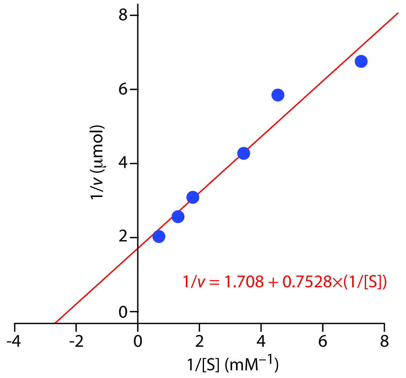
Figure 13.12 Linweaver–Burk plot and regression equation for the data in Example 13.6.
Exercise 13.3
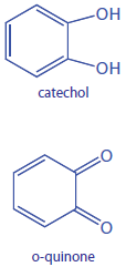 The following data are for the oxidation of catechol (the substrate) to o-quinone by the enzyme o-diphenyl oxidase. The reaction is followed by monitoring the change in absorbance at 540 nm. The data in this exercise are adapted from jkimball.
|
[catechol] (mM) |
0.3 |
0.6 |
1.2 |
4.8 |
|
rate (∆AU/min) |
0.020 |
0.035 |
0.048 |
0.081 |
Determine values for Vmax and Km.
Click here to review your answer to this exercise.
Elucidating Mechanisms for the Inhibition of Enzyme Catalysis
When an inhibitor interacts with an enzyme it decreases the enzyme’s catalytic efficiency. An irreversible inhibitor covalently binds to the enzyme’s active site, producing a permanent loss in catalytic efficiency even if we decrease the inhibitor’s concentration. A reversible inhibitor forms a noncovalent complex with the enzyme, resulting in a temporary decrease in catalytic efficiency. If we remove the inhibitor, the enzyme’s catalytic efficiency returns to its normal level.
There are several pathways for the reversible binding of an inhibitor to an enzyme, as shown in Figure 13.13. In competitive inhibition the substrate and the inhibitor compete for the same active site on the enzyme. Because the substrate cannot bind to an enzyme–inhibitor complex, EI, the enzyme’s catalytic efficiency for the substrate decreases. With noncompetitive inhibition the substrate and the inhibitor bind to different active sites on the enzyme, forming an enzyme–substrate–inhibitor, or ESI complex. The formation of an ESI complex decreases catalytic efficiency because only the enzyme–substrate complex reacts to form the product. Finally, in uncompetitive inhibition the inhibitor binds to the enzyme–substrate complex, forming an inactive ESI complex.
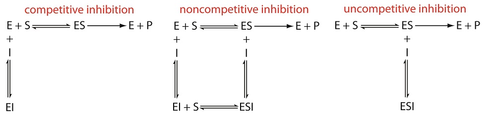
Figure 13.13: Mechanisms for the reversible inhibition of enzyme catalysis. E: enzyme, S: substrate, P: product, I: inhibitor, ES: enzyme–substrate complex, EI: enzyme–inhibitor complex, ESI: enzyme–substrate–inhibitor complex.
We can identify the type of reversible inhibition by observing how a change in the inhibitor’s concentration affects the relationship between the rate of reaction and the substrate’s concentration. As shown in Figure 13.14, when we display kinetic data using as a Lineweaver-Burk plot it is easy to determine which mechanism is in effect. For example, an increase in slope, a decrease in the x-intercept, and no change in the y-intercept indicates competitive inhibition. Because the inhibitor’s binding is reversible, we can still obtain the same maximum velocity—thus the constant value for the y-intercept—by adding enough substrate to completely displace the inhibitor. Because it takes more substrate, the value of Km increases, which explains the increase in the slope and the decrease in the x-intercept’s value.
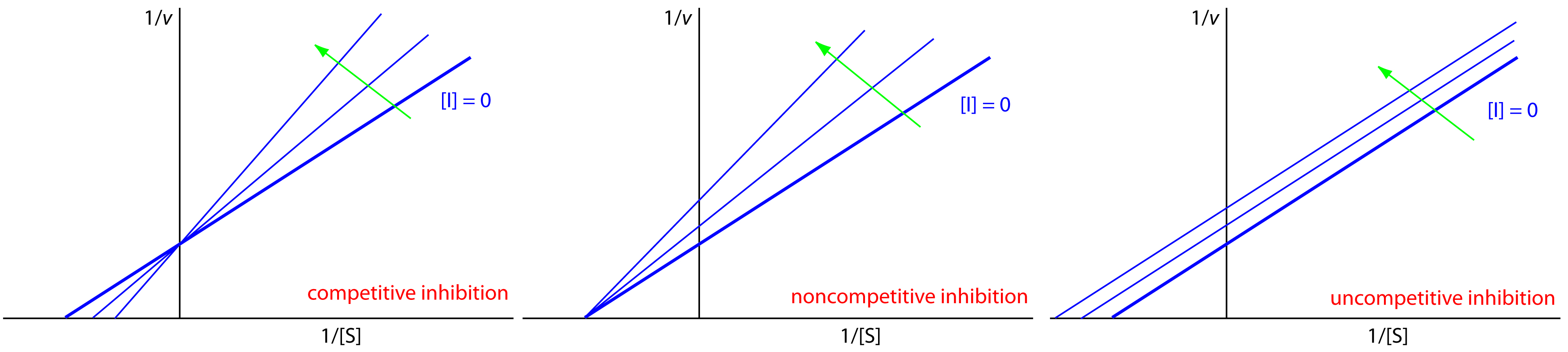
Figure 13.14 Linweaver–Burk plots for competitive inhibition, noncompetitive inhibition, and uncompetitive inhibition. The thick blue line in each plot shows the kinetic behavior in the absence of inhibitor, and the thin blue lines in each plot show the change in behavior for increasing concentrations of the inhibitor. In each plot, the inhibitor’s concentration increases in the direction of the green arrow.
Example 13.7
Practice Exercise 13.3 provides kinetic data for the oxidation of catechol (the substrate) to o-quinone by the enzyme o-diphenyl oxidase in the absence of an inhibitor. The following additional data are available when the reaction is run in the presence of p-hydroxybenzoic acid, PBHA. Is PBHA an inhibitor for this reaction and, if so, what type of inhibitor is it? The data in this exercise are adapted from jkimball.
| [catechol] (mM) | 0.3 | 0.6 | 1.2 | 4.8 |
| rate (∆AU/min) | 0.011 | 0.019 | 0.022 | 0.060 |
Solution
Figure 13.15 shows the resulting Lineweaver–Burk plot for the data in Practice Exercise 13.3 and Example 13.7. Although the y-intercepts are not identical in value—the result of uncertainty in measuring the rates—the plot suggests that PBHA is a competitive inhibitor for the enzyme’s reaction with catechol.
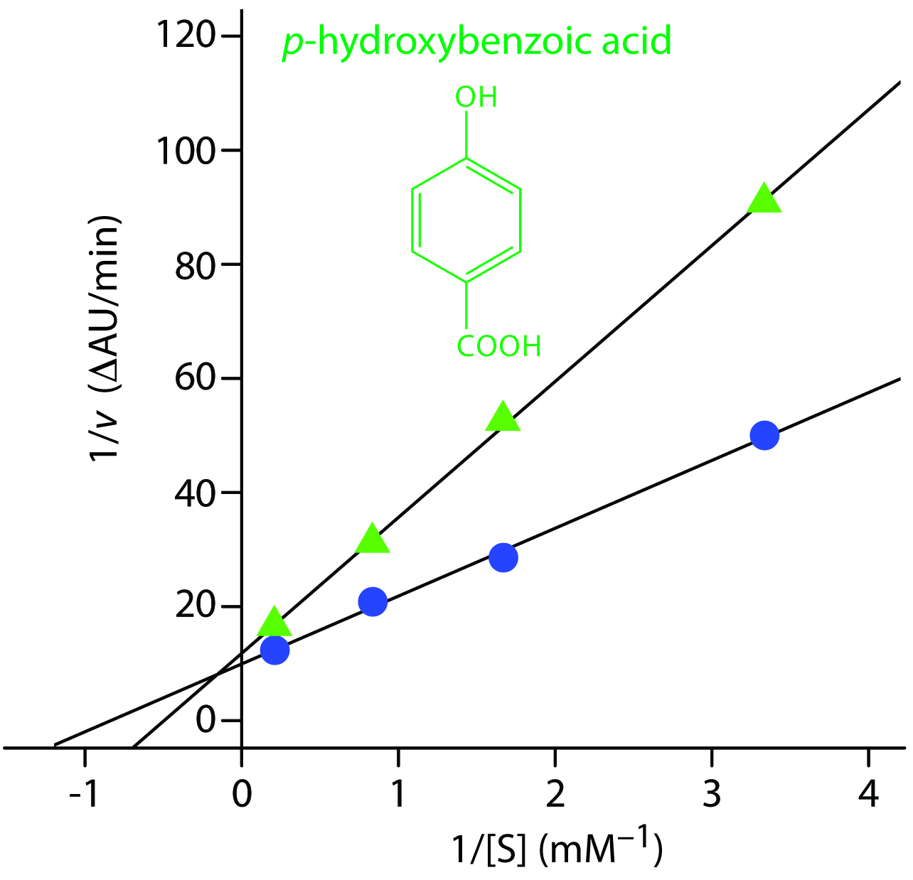
Figure 13.15 Lineweaver–Burk plots for the data in Practice Exercise 13.3 and Example 13.7.
Exercise 13.4
Practice Exercise 13.3 provides kinetic data for the oxidation of catechol (the substrate) to o-quinone by the enzyme o-diphenyl oxidase in the absence of an inhibitor. The following additional data are available when the reaction is run in the presence of phenylthiourea. Is phenylthiourea an inhibitor for this reaction and, if so, what type of inhibitor is it? The data in this exercise are adapted from jkimball.
| [catechol] (mM) | 0.3 | 0.6 | 1.2 | 4.8 |
| rate (∆AU/min) | 0.010 | 0.016 | 0.024 | 0.040 |
Click here to review your answer to this exercise.
13.2.6 Evaluation of Chemical Kinetic Methods
Scale of Operation
The detection limit for chemical kinetic methods ranges from minor components to ultratrace components, and is principally determined by two factors: the rate of the reaction and the instrumental technique used to monitor the rate. Because the signal is directly proportional to the reaction rate, faster reactions generally result in lower detection limits. All other factors being equal, detection limits are smaller for catalytic reactions than for noncatalytic reactions. Not surprisingly, some of the earliest chemical kinetic methods took advantage of catalytic reactions. For example, ultratrace levels of Cu (<1 ppb) can be determined by measuring its catalytic effect on the redox reaction between hydroquinone and H2O2.
See Figure 3.5 to review the meaning of minor, trace, and ultratrace components.
In the absence of a catalyst, most chemical kinetic methods for organic compounds involve reactions with relatively slow rates, limiting the method to minor and higher concentration trace analytes. Noncatalytic chemical kinetic methods for inorganic compounds involving metal–ligand complexation may be fast or slow, with detection limits ranging from trace to minor analyte.
The second factor influencing a method’s detection limit is the instrumental technique used to monitor the reaction’s progress. Most reactions are monitored spectrophotometrically or electrochemically. The scale of operation for these techniques are discussed in Chapter 10 and Chapter 11.
Accuracy
As noted earlier, a chemical kinetic method is potentially subject to larger errors than an equilibrium method due to the effect of uncontrolled or poorly controlled variables, such as temperature or pH. Although a direct-computation chemical kinetic method can achieve moderately accurate results (a relative error of 1–5%), the accuracy often is much worse. Curve-fitting methods may provide significant improvements in accuracy because they use more data. In one study, for example, accuracy was improved by two orders of magnitude—from errors of 500% to 5%—by replacing a direct-computation analysis with a curve-fitting analysis.15 Although not discussed in this chapter, data analysis methods that include the ability to compensate for experimental errors can lead to a significant improvement in accuracy.16
Precision
The precision of a chemical kinetic method is limited by the signal-to-noise ratio of the instrumental technique used to monitor the reaction’s progress. When using an integral method, a precision of 1–2% is routinely possible. The precision for a differential method may be somewhat poorer, particularly when the signal is noisy.
Sensitivity
We can improve the sensitivity of a one-point fixed-time integral method by making measurements under conditions where the concentration of the species we are monitoring is as large as possible. When monitoring the analyte’s concentration—or the concentration of any other reactant—we want to take measurements early in the reaction before its concentration decreases. On the other hand, if we choose to monitor one of the reaction’s products, then it is better to take measurements at longer times. For a two-point fixed-time integral method, we can improve sensitivity by increasing the difference between times t1 and t2. As discussed earlier, the sensitivity of a rate method improves when we choose to measure the initial rate.
Selectivity
The analysis of closely related compounds, as we have seen in earlier chapters, is often complicated by their tendency to interfere with each other. To overcome this problem we usually need to separate the analyte and the interferent before completing the analysis. One advantage of a chemical kinetic method is that we often can adjust the reaction conditions so that the analyte and the interferent have different reaction rates. If the difference in their respective rates is large enough, then one species reacts completely before the other species has a chance to react.
The need to analyze multiple analytes in complex mixtures is, of course, one of the advantages of the separation techniques covered in Chapter 12. Kinetic techniques provide an alternative approach for simple mixtures.
We can use the appropriate integrated rate laws to find the conditions necessary to separate a faster reacting species from a more slowly reacting species. Let’s consider a system consisting of an analyte, A, and an interferent, B, both of which show first-order kinetics with a common reagent. To avoid an interference, the relative magnitudes of their rate constants must be sufficiently different. The fractions, f, of A and B remaining at any point in time, t, are defined by the following equations
\[(f_\ce{A})_t = \dfrac{[\ce A]_t}{[\ce A]_0}\label{13.29}\]
\[(f_\ce{B})_t = \dfrac{[\ce B]_t}{[\ce B]_0}\label{13.30}\]
where [A]0 and [B]0 are the initial concentrations of A and B, respectively. Rearranging Equation \(\ref{13.2}\) and substituting in Equation \(\ref{13.29}\) or Equation \(\ref{13.30}\) leaves use with the following two equations.
\[\ln\dfrac{[\ce A]_t}{[\ce A]_0} = \ln(f_\ce{A})_t = −k_\ce{A}t\label{13.31}\]
\[\ln\dfrac{[\ce B]_t}{[\ce B]_0} = \ln(f_\ce{B})_t = −k_\ce{B}t\label{13.32}\]
where kA and kB are the rate constants for A and B. Dividing Equation \(\ref{13.31}\) by Equation \(\ref{13.32}\) leave us with
\[\dfrac{k_\ce{A}}{k_\ce{B}} = \dfrac{\ln(f_\ce{A})_t}{\ln(f_\ce{B})_t}\]
Suppose we want 99% of A react before 1% of B reacts. The fraction of A that remains is 0.01 and the fraction of B remaining is 0.99, which requires that
\[\dfrac{k_\ce{A}}{k_\ce{B}} = \dfrac{\ln(f_\ce{A})_t}{\ln(f_\ce{B})_t} = \dfrac{\ln(0.01)}{\ln(0.99)} = 460\]
the rate constant for A be at least 460 times larger than that for B. Under these conditions we can determine the analyte’s concentration before the interferent begins to react. If the analyte has the slower reaction, then we can determine its concentration after allowing the interferent to react to completion.
This method of adjusting reaction rates is useful if we need to analyze for an analyte in the presence of an interferent, but impractical if both A and B are analytes because conditions favoring the analysis of A will not favor the analysis of B. For example, if we adjust our conditions so that 99% of A reacts in 5 s, then 99% of B must react within 0.01 s if it has the faster kinetics, or in 2300 s if it has the slower kinetics. The reaction of B is too fast or too slow to make this a useful analytical method.
What do we do if the difference in the rate constants for A and B are not significantly different? We can still complete an analysis if we can simultaneously monitor both species. Because both A and B react at the same time, the integrated form of the first-order rate law becomes
\[C_t = [\ce A]_t + [\ce B]_t = [\ce A]_0e^{−k_\ce{A}t} + [\ce B]_0e^{−k_\ce{B}t}\label{13.33}\]
where Ct is the total concentration of A and B at time, t. If we measure Ct at times t1 and t2, we can solve the resulting pair of simultaneous equations to determine values [A]0 and [B]0. The rate constants kA and kB are determined in separate experiments using standard solutions of A and B.
Equation \(\ref{13.33}\) can also serve as the basis for a curve-fitting method. As shown in Figure 13.16, a plot of ln(Ct) as a function of time consists of two regions. At shorter times the plot is curved because A and B are reacting simultaneously. At later times, however, the concentration of the faster reacting component, A, decreases to zero, and Equation \(\ref{13.33}\) simplifies to
\[C_t ≈ [\ce B]_t = [\ce B]_0e^{−k_\ce{B}t}\]
Under these conditions a plot of ln(Ct) versus time is linear. Extrapolating the linear portion to t = 0 gives [B]0, with [A]0 determined by difference.
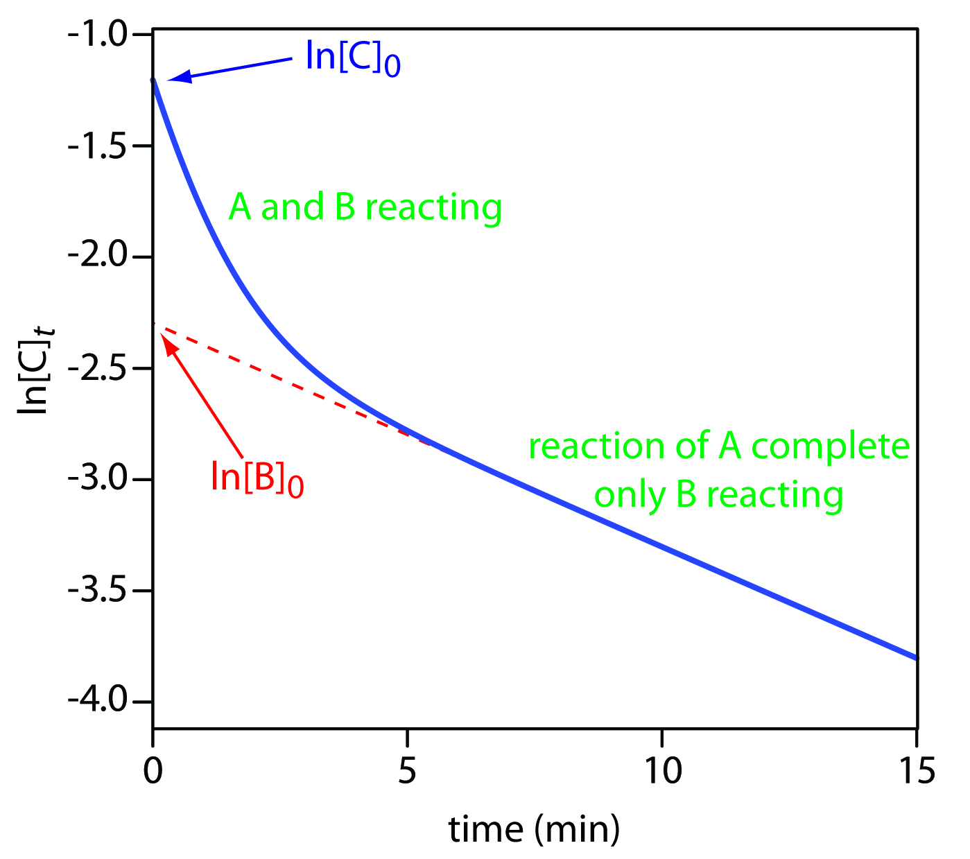
Figure 13.16: Kinetic determination of a slower reacting analyte, B, in the presence of a faster reacting analyte, A. The rate constants for the two analytes are: kA = 1 min–1 and kB = 0.1 min–1. Example 13.8 asks you to use this data to determine the concentrations of A and B in the original sample.
Example 13.8
Use the data in Figure 13.16 to determine the concentrations of A and B in the original sample.
Solution
Extrapolating the linear part of the curve back to t = 0 gives ln[B]0 as –2.3, or a [B]0 of 0.10 M. At t = 0, ln[C]0 is –1.2, corresponding to a [C]0 of 0.30 M. Because [C]0 = [A]0 + [B]0, the concentration of A in the original sample is 0.20 M.
Time, Cost, and Equipment
An automated chemical kinetic method of analysis provides a rapid means for analyzing samples, with throughputs ranging from several hundred to several thousand determinations per hour. The initial start-up costs may be fairly high because an automated analysis requires a dedicated instrument designed to meet the specific needs of the analysis. When measurements are handled manually, a chemical kinetic method requires routinely available equipment and instrumentation, although the sample throughput is much lower than with an automated method.