7.1: The Kinetic-Molecular Theory

Last updated
Save as PDF

Page ID: 395209

\( \newcommand{\vecs}[1]{\overset { \scriptstyle \rightharpoonup} {\mathbf{#1}} } \) \( \newcommand{\vecd}[1]{\overset{-\!-\!\rightharpoonup}{\vphantom{a}\smash {#1}}} \)\(\newcommand{\id}{\mathrm{id}}\) \( \newcommand{\Span}{\mathrm{span}}\) \( \newcommand{\kernel}{\mathrm{null}\,}\) \( \newcommand{\range}{\mathrm{range}\,}\) \( \newcommand{\RealPart}{\mathrm{Re}}\) \( \newcommand{\ImaginaryPart}{\mathrm{Im}}\) \( \newcommand{\Argument}{\mathrm{Arg}}\) \( \newcommand{\norm}[1]{\| #1 \|}\) \( \newcommand{\inner}[2]{\langle #1, #2 \rangle}\) \( \newcommand{\Span}{\mathrm{span}}\) \(\newcommand{\id}{\mathrm{id}}\) \( \newcommand{\Span}{\mathrm{span}}\) \( \newcommand{\kernel}{\mathrm{null}\,}\) \( \newcommand{\range}{\mathrm{range}\,}\) \( \newcommand{\RealPart}{\mathrm{Re}}\) \( \newcommand{\ImaginaryPart}{\mathrm{Im}}\) \( \newcommand{\Argument}{\mathrm{Arg}}\) \( \newcommand{\norm}[1]{\| #1 \|}\) \( \newcommand{\inner}[2]{\langle #1, #2 \rangle}\) \( \newcommand{\Span}{\mathrm{span}}\)\(\newcommand{\AA}{\unicode[.8,0]{x212B}}\)

Learning Objectives

State the postulates of the kinetic-molecular theory
Use this theory’s postulates to explain the gas laws

Steam, water, and ice are often considered three distinct substances because their physical properties are so different. We know that whether water freezes or boils is temperature dependent and this leads to an interesting question: what is temperature? What, exactly, does temperature measure. Temperature is a way to represent the average speed of particles. A lower temperature means molecules are moving slower, while a higher temperature means the molecules are moving faster.

Definition: Absolute Zero

The temperature at which particles have no movement, defined as 0 K or -273.15 °C.

The kinetic-molecular theory (KMT) is a simple molecular model that effectively explains the physical properties of matter using the motion of the molecules. This theory, focusing on gases, is based on the following five postulates described here. (Note: The term “molecule” will be used to refer to the individual chemical species that compose the gas, although some gases are composed of atomic species, for example, the noble gases.)

Gases are composed of molecules that are in continuous motion, travelling in straight lines and changing direction only when they collide with other molecules or with the walls of a container.
The molecules composing the gas are negligibly small compared to the distances between them.
The pressure exerted by a gas in a container results from collisions between the gas molecules and the container walls.
Gas molecules exert no attractive or repulsive forces on each other or the container walls; therefore, their collisions are elastic (do not involve a loss of energy).
The average kinetic energy of the gas molecules is proportional to the kelvin temperature of the gas.

The test of the KMT and its postulates is its ability to explain and describe the behavior of a gas. The various gas laws can be derived from the assumptions of the KMT, which have led chemists to believe that the assumptions of the theory accurately represent the properties of gas molecules. We will first look at the individual gas laws (Boyle’s, Charles’s, Amontons’s, Avogadro’s, and Dalton’s laws) conceptually to see how the KMT explains them. Then, we will more carefully consider the relationships between molecular masses, speeds, and kinetic energies with temperature, and explain Graham’s law.

The Kinetic-Molecular Theory Explains the Behavior of Gases, Part I

Gases consist of rapidly moving gas molecules and, if inside a container, will hit a unit area of the wall per unit of time. The impacts will create pressure in the container. We see that the KMT conceptually explains the behavior of a gas as follows:

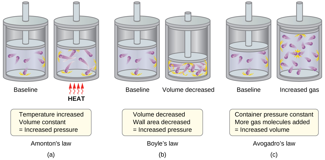
Amontons’s law. If the temperature is increased, the average speed and kinetic energy of the gas molecules increase. If the volume is held constant, the increased speed of the gas molecules results in more frequent and more forceful collisions with the walls of the container, therefore increasing the pressure (Figure \(\PageIndex{1a}\)).
Charles’s law. If the temperature of a gas is increased, a constant pressure may be maintained only if the volume occupied by the gas increases. This will result in greater average distances traveled by the molecules to reach the container walls, as well as increased wall surface area. These conditions will decrease both the frequency of molecule-wall collisions and the number of collisions per unit area, the combined effects of which balance the effect of increased collision forces due to the greater kinetic energy at the higher temperature.
Boyle’s law. If the gas volume is decreased, the container wall area decreases and the molecule-wall collision frequency increases, both of which increase the pressure exerted by the gas (Figure \(\PageIndex{1b}\)).
Avogadro’s law. At constant pressure and temperature, the frequency and force of molecule-wall collisions are constant. Under such conditions, increasing the number of gaseous molecules will require a proportional increase in the container volume in order to yield a decrease in the number of collisions per unit area to compensate for the increased frequency of collisions (Figure \(\PageIndex{1c}\)).
Dalton’s Law. Because of the large distances between them, the molecules of one gas in a mixture bombard the container walls with the same frequency whether other gases are present or not, and the total pressure of a gas mixture equals the sum of the (partial) pressures of the individual gases.

This figure shows 3 pairs of pistons and cylinders. In a, which is labeled, “Charles’s Law,” the piston is positioned for the first cylinder so that just over half of the available volume contains 6 purple spheres with trails behind them. The trails indicate movement. Orange dashes extend from the interior surface of the cylinder where the spheres have collided. This cylinder is labeled, “Baseline.” In the second cylinder, the piston is in the same position, and the label, “Heat” is indicated in red capitalized text. Four red arrows with wavy stems are pointing upward to the base of the cylinder. The six purple spheres have longer trails behind them and the number of orange dashes indicating points of collision with the container walls has increased. A rectangle beneath the diagram states, “Temperature increased, Volume constant equals Increased pressure.” In b, which is labeled, “Boyle’s Law,” the first, baseline cylinder shown is identical to the first cylinder in a. In the second cylinder, the piston has been moved, decreasing the volume available to the 6 purple spheres to half of the initial volume. The six purple spheres have longer trails behind them and the number of orange dashes indicating points of collision with the container walls has increased. This second cylinder is labeled, “Volume decreased.” A rectangle beneath the diagram states, “Volume decreased, Wall area decreased equals Increased pressure.” In c, which is labeled “Avogadro’s Law,” the first, baseline cylinder shown is identical to the first cylinder in a. In the second cylinder, the number of purple spheres has changed from 6 to 12 and volume has doubled. This second cylinder is labeled “Increased gas.” A rectangle beneath the diagram states, “At constant pressure, More gas molecules added equals Increased volume.” — Figure \(\PageIndex{1}\): (a) When gas temperature increases, gas pressure increases due to increased force and frequency of molecular collisions. (b) When volume decreases, gas pressure increases due to increased frequency of molecular collisions. (c) When the amount of gas increases at a constant pressure, volume increases to yield a constant number of collisions per unit wall area per unit time.

Molecular Velocities and Kinetic Energy

The previous discussion showed that the KMT qualitatively explains the behaviors described by the various gas laws. The postulates of this theory may be applied in a more quantitative fashion to derive these individual laws. To do this, we must first look at velocities and kinetic energies of gas molecules, and the temperature of a gas sample.

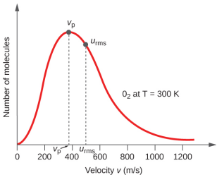
In a gas sample, individual molecules have widely varying speeds; however, because of the vast number of molecules and collisions involved, the molecular speed distribution and average speed are constant. This molecular speed distribution is known as a Maxwell-Boltzmann distribution, and it depicts the relative numbers of molecules in a bulk sample of gas that possesses a given speed (Figure \(\PageIndex{2}\)).

alt — Figure \(\PageIndex{2}\): The molecular speed distribution for oxygen gas at 300 K is shown here. Very few molecules move at either very low or very high speeds. The number of molecules with intermediate speeds increases rapidly up to a maximum, which is the most probable speed, then drops off rapidly. Note that the most probable speed, ν_p, is a little less than 400 m/s, while the root mean square speed, u_rms, is closer to 500 m/s.

The kinetic energy (KE) of a particle of mass (m) and speed (v) is given by:

\[\ce{KE}=\dfrac{1}{2}mv^2 \nonumber \]

Expressing mass in kilograms and speed in meters per second will yield energy values in units of joules (J = kg m² s^–2). To deal with a large number of gas molecules, we use averages for both speed and kinetic energy. In the KMT, the root mean square velocity of a particle, u_rms, is defined as the square root of the average of the squares of the velocities with n = the number of particles:

\[u_\ce{rms}=\sqrt{\overline{u^2}}=\sqrt{\dfrac{v^2_1+v^2_2+v^2_3+v^2_4+…}{n}} \nonumber \]

The average kinetic energy, KE_avg, is then equal to:

\[\mathrm{KE_{avg}}=\dfrac{1}{2}mv^2_\ce{rms} \nonumber \]

The KE_avg of a collection of gas molecules is also directly proportional to the temperature of the gas and may be described by the equation:

\[\mathrm{KE_{avg}}\propto T \nonumber \]

where we can then substitute kinetic energy and see

\[\mathrm{mv^2_{avg}}\propto T \nonumber \]

The average velocity of the molecules is inverse to the mass of the molecule, assuming temperature is constant. Similarly, we can see that velocity increases with temperature, assuming mass is constant.

Example \(\PageIndex{1}\): Determining the relative velocity of a molecule

Order the following gases at the same temperature from least relative velocity to greatest relative velocity: oxygen gas, chlorine gas, hydrogen gas.

Solution

Determine the formula mass of each molecule. Oxygen gas is 32 amu, chlorine gas is 71 amu, and hydrogen gas is 1.0 amu. Mass is inversely proportional to mass, thus the order from least to greatest will be the opposite of the masses.

\[\text{Least}\ \rightarrow\ \text{Greatest}\]

\[\text{Mass}\]

\[\text{hydrogen}\ \rightarrow\ \text{oxygen}\ \rightarrow\ \text{chlorine}\]

\[\text{Relative Velocity}\]

\[\text{chlorine}\ \rightarrow\ \text{oxygen}\ \rightarrow\ \text{hydrogen}\]

Exercise \(\PageIndex{1}\)

Order the following gases at the same temperature from least relative velocity to greatest relative velocity: bromine gas, fluorine gas, and helium gas.

Answer: \(\text{bromine}\ \rightarrow\ \text{fluorine}\ \rightarrow\ \text{helium}\)

If the temperature of a gas increases, its KE_avg increases, more molecules have higher speeds and fewer molecules have lower speeds, and the distribution shifts toward higher speeds overall, that is, to the right. If temperature decreases, KE_avg decreases, more molecules have lower speeds and fewer molecules have higher speeds, and the distribution shifts toward lower speeds overall, that is, to the left. This behavior is illustrated for nitrogen gas in Figure \(\PageIndex{3}\).

A graph with four positively or right-skewed curves of varying heights is shown. The horizontal axis is labeled, “Velocity v ( m divided by s ).” This axis is marked by increments of 500 beginning at 0 and extending up to 1500. The vertical axis is labeled, “Fraction of molecules.” The label, “N subscript 2,” appears in the open space in the upper right area of the graph. The tallest and narrowest of these curves is labeled, “100 K.” Its right end appears to touch the horizontal axis around 700 m per s. It is followed by a slightly wider curve which is labeled, “200 K,” that is about three quarters of the height of the initial curve. Its right end appears to touch the horizontal axis around 850 m per s. The third curve is significantly wider and only about half the height of the initial curve. It is labeled, “500 K.” Its right end appears to touch the horizontal axis around 1450 m per s. The final curve is only about one third the height of the initial curve. It is much wider than the others, so much so that its right end has not yet reached the horizontal axis. This curve is labeled, “1000 K.” — Figure \(\PageIndex{3}\): The molecular speed distribution for nitrogen gas (N₂) shifts to the right and flattens as the temperature increases; it shifts to the left and heightens as the temperature decreases.

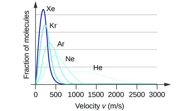
At a given temperature, all gases have the same KE_avg for their molecules. Gases composed of lighter molecules have more high-speed particles and a higher u_rms, with a speed distribution that peaks at relatively higher velocities. Gases consisting of heavier molecules have more low-speed particles, a lower u_rms, and a speed distribution that peaks at relatively lower velocities. This trend is demonstrated by the data for a series of noble gases shown in Figure \(\PageIndex{4}\).

A graph is shown with four positively or right-skewed curves of varying heights. The horizontal axis is labeled, “Velocity v ( m divided by s ).” This axis is marked by increments of 500 beginning at 0 and extending up to 3000. The vertical axis is labeled, “Fraction of molecules.” The tallest and narrowest of these curves is labeled, “X e.” Its right end appears to touch the horizontal axis around 600 m per s. It is followed by a slightly wider curve which is labeled, “A r,” that is about half the height of the initial curve. Its right end appears to touch the horizontal axis around 900 m per s. The third curve is significantly wider and just over a third of the height of the initial curve. It is labeled, “N e.” Its right end appears to touch the horizontal axis around 1200 m per s. The final curve is only about one fourth the height of the initial curve. It is much wider than the others, so much so that its right reaches the horizontal axis around 2500 m per s. This curve is labeled, “H e.” — Figure \(\PageIndex{4}\): Molecular velocity is directly related to molecular mass. At a given temperature, lighter molecules move faster on average than heavier molecules.

The Kinetic-Molecular Theory Explains the Behavior of Gases, Part II

The molecules of a gas are in rapid motion and the molecules themselves are small. The average distance between the molecules of a gas is large compared to the size of the molecules. As a consequence, gas molecules can move past each other easily and diffuse at relatively fast rates.

The rate of effusion of a gas depends directly on the (average) speed of its molecules:

\[\textrm{effusion rate} ∝ v_\ce{rms} \nonumber \]

Using this relation, and the equation relating molecular speed to mass, Graham’s law may be easily derived as shown here:

\[u_\ce{rms}=\sqrt{\dfrac{3RT}{m}} \nonumber \]

\[m=\dfrac{3RT}{u^2_\ce{rms}}=\dfrac{3RT}{\overline{u}^2} \nonumber \]

\[\mathrm{\dfrac{effusion\: rate\: A}{effusion\: rate\: B}}=\dfrac{u_\mathrm{rms\:A}}{u_\mathrm{rms\:B}}=\dfrac{\sqrt{\dfrac{3RT}{m_\ce{A}}}}{\sqrt{\dfrac{3RT}{m_\ce{B}}}}=\sqrt{\dfrac{m_\ce{B}}{m_\ce{A}}} \nonumber \]

The ratio of the rates of effusion is thus derived to be inversely proportional to the ratio of the square roots of their masses.

Kinetic-Molecular Theory of Gases: https://youtu.be/9f83XAYfXAg

Summary

The kinetic molecular theory is a simple but very effective model that effectively explains ideal gas behavior. The theory assumes that gases consist of widely separated molecules of negligible volume that are in constant motion, colliding elastically with one another and the walls of their container with average velocities determined by their absolute temperatures. The individual molecules of a gas exhibit a range of velocities, the distribution of these velocities being dependent on the temperature of the gas and the mass of its molecules.

Key Equations

\(\mathrm{KE_{avg}}\propto T \nonumber \)
\(\mathrm{mv^2_{avg}}\propto T \nonumber \)

Summary

kinetic molecular theory: theory based on simple principles and assumptions that effectively explains the properties of states of matter