5.4: The Kinetic-Molecular Theory, Effusion, and Diffusion

Learning Objectives

• State the postulates of the kinetic-molecular theory
• Use this theory’s postulates to explain the gas laws
• Define and explain effusion and diffusion
• State Graham’s law and use it to compute relevant gas properties

The gas laws that we have seen to this point, as well as the ideal gas equation, are empirical, that is, they have been derived from experimental observations. The mathematical forms of these laws closely describe the macroscopic behavior of most gases at pressures less than about 1 or 2 atm. Although the gas laws describe relationships that have been verified by many experiments, they do not tell us why gases follow these relationships.

The kinetic molecular theory (KMT) is a simple microscopic model that effectively explains the gas laws described in previous modules of this chapter. This theory is based on the following five postulates described here. (Note: The term “molecule” will be used to refer to the individual chemical species that compose the gas, although some gases are composed of atomic species, for example, the noble gases.)

1. Gases are composed of molecules that are in continuous motion, travelling in straight lines and changing direction only when they collide with other molecules or with the walls of a container.
2. The molecules composing the gas are negligibly small compared to the distances between them.
3. The pressure exerted by a gas in a container results from collisions between the gas molecules and the container walls.
4. Gas molecules exert no attractive or repulsive forces on each other or the container walls; therefore, their collisions are elastic (do not involve a loss of energy).
5. The average kinetic energy of the gas molecules is proportional to the kelvin temperature of the gas.

The test of the KMT and its postulates is its ability to explain and describe the behavior of a gas. The various gas laws can be derived from the assumptions of the KMT, which have led chemists to believe that the assumptions of the theory accurately represent the properties of gas molecules. We will first look at the individual gas laws (Boyle’s, Charles’s, Amontons’s, Avogadro’s, and Dalton’s laws) conceptually to see how the KMT explains them. Then, we will more carefully consider the relationships between molecular masses, speeds, and kinetic energies with temperature, and explain Graham’s law.

The Kinetic-Molecular Theory Explains the Behavior of Gases, Part I

Recalling that gas pressure is exerted by rapidly moving gas molecules and depends directly on the number of molecules hitting a unit area of the wall per unit of time, we see that the KMT conceptually explains the behavior of a gas as follows:

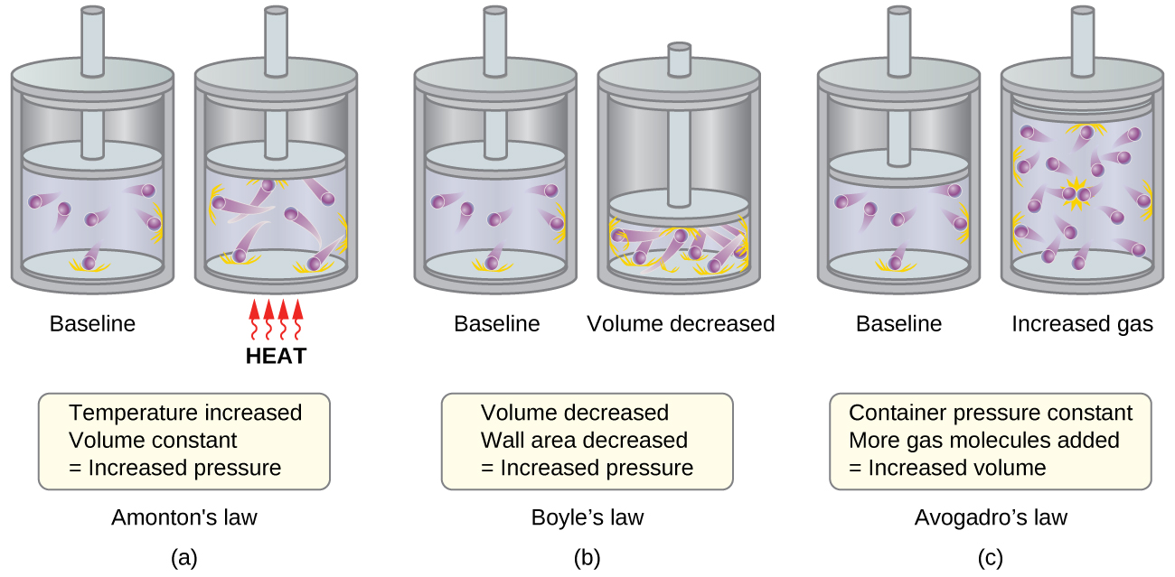
• Amontons’s law. If the temperature is increased, the average speed and kinetic energy of the gas molecules increase. If the volume is held constant, the increased speed of the gas molecules results in more frequent and more forceful collisions with the walls of the container, therefore increasing the pressure (Figure \(\PageIndex{1a}\)).
• Charles’s law. If the temperature of a gas is increased, a constant pressure may be maintained only if the volume occupied by the gas increases. This will result in greater average distances traveled by the molecules to reach the container walls, as well as increased wall surface area. These conditions will decrease both the frequency of molecule-wall collisions and the number of collisions per unit area, the combined effects of which balance the effect of increased collision forces due to the greater kinetic energy at the higher temperature.
• Boyle’s law. If the gas volume is decreased, the container wall area decreases and the molecule-wall collision frequency increases, both of which increase the pressure exerted by the gas (Figure \(\PageIndex{1b}\)).
• Avogadro’s law. At constant pressure and temperature, the frequency and force of molecule-wall collisions are constant. Under such conditions, increasing the number of gaseous molecules will require a proportional increase in the container volume in order to yield a decrease in the number of collisions per unit area to compensate for the increased frequency of collisions (Figure \(\PageIndex{1c}\)).
• Dalton’s Law. Because of the large distances between them, the molecules of one gas in a mixture bombard the container walls with the same frequency whether other gases are present or not, and the total pressure of a gas mixture equals the sum of the (partial) pressures of the individual gases.

Figure \(\PageIndex{1}\): (a) When gas temperature increases, gas pressure increases due to increased force and frequency of molecular collisions. (b) When volume decreases, gas pressure increases due to increased frequency of molecular collisions. (c) When the amount of gas increases at a constant pressure, volume increases to yield a constant number of collisions per unit wall area per unit time.

Molecular Velocities and Kinetic Energy

The previous discussion showed that the KMT qualitatively explains the behaviors described by the various gas laws. The postulates of this theory may be applied in a more quantitative fashion to derive these individual laws. To do this, we must first look at velocities and kinetic energies of gas molecules, and the temperature of a gas sample.

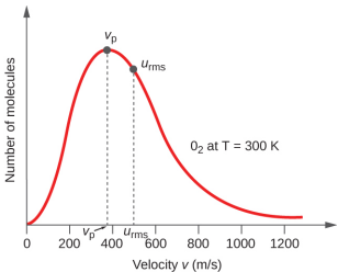
In a gas sample, individual molecules have widely varying speeds; however, because of the vast number of molecules and collisions involved, the molecular speed distribution and average speed are constant. This molecular speed distribution is known as a Maxwell-Boltzmann distribution, and it depicts the relative numbers of molecules in a bulk sample of gas that possesses a given speed (Figure \(\PageIndex{2}\)).

Figure \(\PageIndex{2}\): The molecular speed distribution for oxygen gas at 300 K is shown here. Very few molecules move at either very low or very high speeds. The number of molecules with intermediate speeds increases rapidly up to a maximum, which is the most probable speed, then drops off rapidly. Note that the most probable speed, ν_p, is a little less than 400 m/s, while the root mean square speed, u_rms, is closer to 500 m/s.

The kinetic energy (KE) of a particle of mass (m) and speed (u) is given by:

\[\ce{KE}=\dfrac{1}{2}mu^2\]

Expressing mass in kilograms and speed in meters per second will yield energy values in units of joules (J = kg m² s^–2). Since there are a very large number of gas molecules in a sample, the average speed and kinetic energy are used for calculations. In kinetic molecular theory the average kinetic energy for a system is calculated using the root mean square velocity of the particles, u_rms so that the average kinetic energy, KE_avg, is then equal to:

\[\mathrm{KE_{avg}}=\dfrac{1}{2}mu^2_\ce{rms}\]

The KE_avg of a collection of gas molecules is also directly proportional to the temperature of the gas and may be described by the equation:

\[\mathrm{KE_{avg}}=\dfrac{3}{2}RT\]

where R is the gas constant, R = 8.314 J mol^-1K^-1, and T is the kelvin temperature. This form of the gas law constant is used since the joule (J) is also the unit for energy.  Combining and rearranging these equations gives the relationship between molecular speed and temperature:

\[u_\ce{rms}=\sqrt{\dfrac{3RT}{m}} \label{RMS}\]

Example \(\PageIndex{1}\): Calculation of u_rms

Calculate the root-mean-square velocity for a nitrogen molecule at 30 °C.

Solution

Convert the temperature into Kelvin:

\[30°C+273=303\: K \nonumber\]

Determine the mass of a nitrogen molecule in kilograms:

\[\mathrm{\dfrac{28.0\cancel{g}}{1\: mol}×\dfrac{1\: kg}{1000\cancel{g}}=0.028\:kg/mol} \nonumber\]

Replace the variables and constants in the root-mean-square velocity formula (Equation \ref{RMS}), replacing Joules with the equivalent kg m²s^–2:

\[ \begin{align*} u_\ce{rms} &= \sqrt{\dfrac{3RT}{m}} \\ u_\ce{rms} &=\sqrt{\dfrac{3(8.314\:J/mol\: K)(303\: K)}{(0.028\:kg/mol)}} \\ &=\sqrt{2.70 \times 10^5\:m^2s^{−2}} \\ &= 519\:m/s \end{align*} \]

Exercise \(\PageIndex{1}\)

Calculate the root-mean-square velocity for an oxygen molecule at –23 °C.

Answer

441 m/s

If the temperature of a gas increases, its KE_avg increases, more molecules have higher speeds and fewer molecules have lower speeds, and the distribution shifts toward higher speeds overall, that is, to the right. If temperature decreases, KE_avg decreases, more molecules have lower speeds and fewer molecules have higher speeds, and the distribution shifts toward lower speeds overall, that is, to the left. This behavior is illustrated for nitrogen gas in Figure \(\PageIndex{3}\).

Figure \(\PageIndex{3}\): The molecular speed distribution for nitrogen gas (N₂) shifts to the right and flattens as the temperature increases; it shifts to the left and heightens as the temperature decreases.

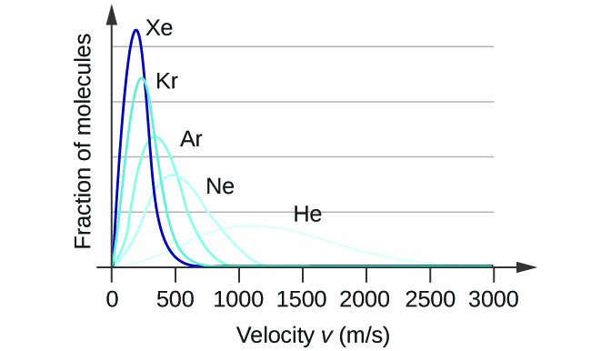
At a given temperature, all gases have the same KE_avg for their molecules. Gases composed of lighter molecules have more high-speed particles and a higher u_rms, with a speed distribution that peaks at relatively higher velocities. Gases consisting of heavier molecules have more low-speed particles, a lower u_rms, and a speed distribution that peaks at relatively lower velocities. This trend is demonstrated by the data for a series of noble gases shown in Figure \(\PageIndex{4}\).

Figure \(\PageIndex{4}\): Molecular velocity is directly related to molecular mass. At a given temperature, lighter molecules move faster on average than heavier molecules.

The PhET gas simulator may be used to examine the effect of temperature on molecular velocities. Examine the simulator’s “energy histograms” (molecular speed distributions) and “species information” (which gives average speed values) for molecules of different masses at various temperatures.

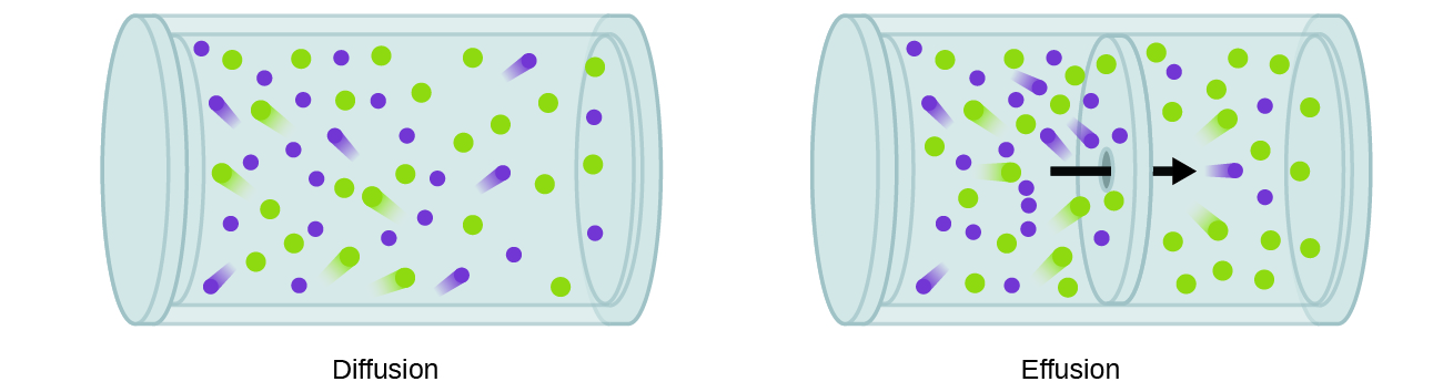
Diffusion

If you have ever been in a room when a piping hot pizza was delivered, you have been made aware of the fact that gaseous molecules can quickly spread throughout a room, as evidenced by the pleasant aroma that soon reaches your nose. Although gaseous molecules travel at tremendous speeds (hundreds of meters per second), they collide with other gaseous molecules and travel in many different directions before reaching the desired target. At room temperature, a gaseous molecule will experience billions of collisions per second. The mean free path is the average distance a molecule travels between collisions. The mean free path increases as pressure is reduced; in general, the mean free path for a gaseous molecule will be hundreds of times the diameter of the molecule

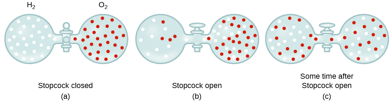
In general, we know that when a sample of gas is introduced to one part of a closed container, its molecules very quickly disperse throughout the container; this process by which molecules disperse in space in response to differences in concentration is called diffusion (shown in Figure \(\PageIndex{5}\)). The gaseous atoms or molecules are, of course, unaware of any concentration gradient, they simply move randomly—regions of higher concentration have more particles than regions of lower concentrations, and so a net movement of species from high to low concentration areas takes place. In a closed environment, diffusion ultimately results in equal concentrations of gas throughout the system. When the concentrations are equal the system is at equilibrium.  Although the gaseous atoms and molecules continue to move, the concentrations is the same in both bulbs so the rates of molecules going in and out of each flask are the same so no net transfer of molecules occurs.

Figure \(\PageIndex{5}\): (a) Two gases, H₂ and O₂, are initially separated. (b) When the stopcock is opened, they mix together. The lighter gas, H₂, passes through the opening faster than O₂, so just after the stopcock is opened, more H₂ molecules move to the O₂ side than O₂ molecules move to the H₂ side. (c) After a short time, both the slower-moving O₂ molecules and the faster-moving H₂ molecules have distributed themselves evenly on both sides of the vessel.

We are often interested in the rate of diffusion, the amount of gas passing through some area per unit time:

\[\textrm{rate of diffusion}=\dfrac{\textrm{amount of gas passing through an area}}{\textrm{unit of time}}\]

The diffusion rate depends on several factors: the concentration gradient (the increase or decrease in concentration from one point to another); the amount of surface area available for diffusion; and the distance the gas particles must travel. Note also that the time required for diffusion to occur is inversely proportional to the rate of diffusion, as shown in the rate of diffusion equation.

A process involving movement of gaseous species similar to diffusion is effusion, the escape of gas molecules through a tiny hole such as a pinhole in a balloon into a vacuum (Figure \(\PageIndex{6}\)). Although diffusion and effusion rates both depend on the molar mass of the gas involved, their rates are not equal; however, the ratios of their rates are the same.

Figure \(\PageIndex{6}\): Diffusion occurs when gas molecules disperse throughout a container. Effusion occurs when a gas passes through an opening that is smaller than the mean free path of the particles, that is, the average distance traveled between collisions. Effectively, this means that only one particle passes through at a time.

If a mixture of gases is placed in a container with porous walls, the gases effuse through the small openings in the walls. The lighter gases pass through the small openings more rapidly (at a higher rate) than the heavier ones (Figure \(\PageIndex{2}\)). In 1832, Thomas Graham studied the rates of effusion of different gases and formulated Graham’s law of effusion: The rate of effusion of a gas is inversely proportional to the square root of the mass of its particles:

\[\textrm{rate of effusion}∝\dfrac{1}{\sqrt{ℳ}}\]

This means that if two gases A and B are at the same temperature and pressure, the ratio of their effusion rates is inversely proportional to the ratio of the square roots of the masses of their particles:

\[\dfrac{\textrm{rate of effusion of B}}{\textrm{rate of effusion of A}}=\dfrac{\sqrt{ℳ_\ce{B}}}{\sqrt{ℳ_\ce{A}}}\]

Figure \(\PageIndex{7}\): A balloon filled with air (the blue one) remains full overnight. A balloon filled with helium (the green one) partially deflates because the smaller, light helium atoms effuse through small holes in the rubber much more readily than the heavier molecules of nitrogen and oxygen found in air. (credit: modification of work by Mark Ott)

 

Application: Use of Diffusion for Uranium Enrichment

Gaseous diffusion has been used to produce enriched uranium for use in nuclear power plants and weapons. Naturally occurring uranium contains only 0.72% of ²³⁵U, the kind of uranium that is “fissile,” that is, capable of sustaining a nuclear fission chain reaction. Nuclear reactors require fuel that is 2–5% ²³⁵U, and nuclear bombs need even higher concentrations. One way to enrich uranium to the desired levels is to take advantage of Graham’s law. In a gaseous diffusion enrichment plant, uranium hexafluoride (UF₆, the only uranium compound that is volatile enough to work) is slowly pumped through large cylindrical vessels called diffusers, which contain porous barriers with microscopic openings. The process is one of diffusion because the other side of the barrier is not evacuated. The ²³⁵UF₆ molecules have a higher average speed and diffuse through the barrier a little faster than the heavier ²³⁸UF₆ molecules. The gas that has passed through the barrier is slightly enriched in ²³⁵UF₆ and the residual gas is slightly depleted. The small difference in molecular weights between ²³⁵UF₆ and ²³⁸UF₆ only about 0.4% enrichment, is achieved in one diffuser (Figure \(\PageIndex{8}\)). But by connecting many diffusers in a sequence of stages (called a cascade), the desired level of enrichment can be attained.

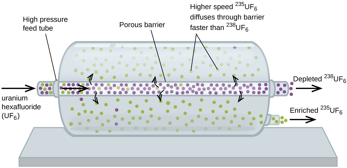
Figure \(\PageIndex{8}\): In a diffuser, gaseous UF₆ is pumped through a porous barrier, which partially separates ²³⁵UF₆ from ²³⁸UF₆ The UF₆ must pass through many large diffuser units to achieve sufficient enrichment in ²³⁵U.

The large scale separation of gaseous ²³⁵UF₆ from ²³⁸UF₆ was first done during the World War II, at the atomic energy installation in Oak Ridge, Tennessee, as part of the Manhattan Project (the development of the first atomic bomb). Although the theory is simple, this required surmounting many daunting technical challenges to make it work in practice. The barrier must have tiny, uniform holes (about 10^–6 cm in diameter) and be porous enough to produce high flow rates. All materials (the barrier, tubing, surface coatings, lubricants, and gaskets) need to be able to contain, but not react with, the highly reactive and corrosive UF₆.

Summary

The kinetic molecular theory is a simple but very effective model that effectively explains ideal gas behavior. The theory assumes that gases consist of widely separated molecules of negligible volume that are in constant motion, colliding elastically with one another and the walls of their container with average velocities determined by their absolute temperatures. The individual molecules of a gas exhibit a range of velocities, the distribution of these velocities being dependent on the temperature of the gas and the mass of its molecules.

Gaseous atoms and molecules move freely and randomly through space. Diffusion is the process whereby gaseous atoms and molecules are transferred from regions of relatively high concentration to regions of relatively low concentration. Effusion is a similar process in which gaseous species pass from a container to a vacuum through very small orifices. The rates of effusion of gases are inversely proportional to the square roots of their densities or to the square roots of their atoms/molecules’ masses (Graham’s law).

Key Equations

• \(u_\ce{rms}=\sqrt{\overline{u^2}}=\sqrt{\dfrac{u^2_1+u^2_2+u^2_3+u^2_4+…}{n}}\)
• \(\mathrm{KE_{avg}}=\dfrac{3}{2}RT\)
• \(u_\ce{rms}=\sqrt{\dfrac{3RT}{m}}\)
• \(\textrm{rate of diffusion}=\dfrac{\textrm{amount of gas passing through an area}}{\textrm{unit of time}}\)
• \(\dfrac{\textrm{rate of effusion of gas B}}{\textrm{rate of effusion of gas A}}=\dfrac{\sqrt{m_B}}{\sqrt{m_A}}=\dfrac{\sqrt{ℳ_B}}{\sqrt{ℳ_A}}\)

Glossary

 

kinetic molecular theory

theory based on simple principles and assumptions that effectively explains ideal gas behavior

root mean square velocity (u_rms)

measure of average velocity for a group of particles calculated as the square root of the average squared velocity

diffusion

movement of an atom or molecule from a region of relatively high concentration to one of relatively low concentration (discussed in this chapter with regard to gaseous species, but applicable to species in any phase)

effusion

transfer of gaseous atoms or molecules from a container to a vacuum through very small openings

Graham’s law of effusion

rates of diffusion and effusion of gases are inversely proportional to the square roots of their molecular masses

mean free path

average distance a molecule travels between collisions

rate of diffusion

amount of gas diffusing through a given area over a given time

Contributors and Attributions

• {{Template.ContribOpenStax()}

• Paul Flowers (University of North Carolina - Pembroke), Klaus Theopold (University of Delaware) and Richard Langley (Stephen F. Austin State University) with contributing authors. Textbook content produced by OpenStax College is licensed under a Creative Commons Attribution License 4.0 license. Download for free at http://cnx.org/contents/85abf193-2bd...a7ac8df6@9.110).