8.2: Collision Theory and Reaction Mechanisms

Last updated
Save as PDF

Page ID: 431440

$ \newcommand{\vecs}[1]{\overset { \scriptstyle \rightharpoonup} {\mathbf{#1}} } $

$ \newcommand{\vecd}[1]{\overset{-\!-\!\rightharpoonup}{\vphantom{a}\smash {#1}}} $

$ \newcommand{\id}{\mathrm{id}}$ $ \newcommand{\Span}{\mathrm{span}}$

( \newcommand{\kernel}{\mathrm{null}\,}\) $ \newcommand{\range}{\mathrm{range}\,}$

$ \newcommand{\RealPart}{\mathrm{Re}}$ $ \newcommand{\ImaginaryPart}{\mathrm{Im}}$

$ \newcommand{\Argument}{\mathrm{Arg}}$ $ \newcommand{\norm}[1]{\| #1 \|}$

$ \newcommand{\inner}[2]{\langle #1, #2 \rangle}$

$ \newcommand{\Span}{\mathrm{span}}$

$ \newcommand{\id}{\mathrm{id}}$

$ \newcommand{\Span}{\mathrm{span}}$

$ \newcommand{\kernel}{\mathrm{null}\,}$

$ \newcommand{\range}{\mathrm{range}\,}$

$ \newcommand{\RealPart}{\mathrm{Re}}$

$ \newcommand{\ImaginaryPart}{\mathrm{Im}}$

$ \newcommand{\Argument}{\mathrm{Arg}}$

$ \newcommand{\norm}[1]{\| #1 \|}$

$ \newcommand{\inner}[2]{\langle #1, #2 \rangle}$

$ \newcommand{\Span}{\mathrm{span}}$ $ \newcommand{\AA}{\unicode[.8,0]{x212B}}$

$ \newcommand{\vectorA}[1]{\vec{#1}} % arrow$

$ \newcommand{\vectorAt}[1]{\vec{\text{#1}}} % arrow$

$ \newcommand{\vectorB}[1]{\overset { \scriptstyle \rightharpoonup} {\mathbf{#1}} } $

$ \newcommand{\vectorC}[1]{\textbf{#1}} $

$ \newcommand{\vectorD}[1]{\overrightarrow{#1}} $

$ \newcommand{\vectorDt}[1]{\overrightarrow{\text{#1}}} $

$ \newcommand{\vectE}[1]{\overset{-\!-\!\rightharpoonup}{\vphantom{a}\smash{\mathbf {#1}}}} $

$ \newcommand{\vecs}[1]{\overset { \scriptstyle \rightharpoonup} {\mathbf{#1}} } $

$ \newcommand{\vecd}[1]{\overset{-\!-\!\rightharpoonup}{\vphantom{a}\smash {#1}}} $

$\newcommand{\avec}{\mathbf a}$ $\newcommand{\bvec}{\mathbf b}$ $\newcommand{\cvec}{\mathbf c}$ $\newcommand{\dvec}{\mathbf d}$ $\newcommand{\dtil}{\widetilde{\mathbf d}}$ $\newcommand{\evec}{\mathbf e}$ $\newcommand{\fvec}{\mathbf f}$ $\newcommand{\nvec}{\mathbf n}$ $\newcommand{\pvec}{\mathbf p}$ $\newcommand{\qvec}{\mathbf q}$ $\newcommand{\svec}{\mathbf s}$ $\newcommand{\tvec}{\mathbf t}$ $\newcommand{\uvec}{\mathbf u}$ $\newcommand{\vvec}{\mathbf v}$ $\newcommand{\wvec}{\mathbf w}$ $\newcommand{\xvec}{\mathbf x}$ $\newcommand{\yvec}{\mathbf y}$ $\newcommand{\zvec}{\mathbf z}$ $\newcommand{\rvec}{\mathbf r}$ $\newcommand{\mvec}{\mathbf m}$ $\newcommand{\zerovec}{\mathbf 0}$ $\newcommand{\onevec}{\mathbf 1}$ $\newcommand{\real}{\mathbb R}$ $\newcommand{\twovec}[2]{\left[\begin{array}{r}#1 \\ #2 \end{array}\right]}$ $\newcommand{\ctwovec}[2]{\left[\begin{array}{c}#1 \\ #2 \end{array}\right]}$ $\newcommand{\threevec}[3]{\left[\begin{array}{r}#1 \\ #2 \\ #3 \end{array}\right]}$ $\newcommand{\cthreevec}[3]{\left[\begin{array}{c}#1 \\ #2 \\ #3 \end{array}\right]}$ $\newcommand{\fourvec}[4]{\left[\begin{array}{r}#1 \\ #2 \\ #3 \\ #4 \end{array}\right]}$ $\newcommand{\cfourvec}[4]{\left[\begin{array}{c}#1 \\ #2 \\ #3 \\ #4 \end{array}\right]}$ $\newcommand{\fivevec}[5]{\left[\begin{array}{r}#1 \\ #2 \\ #3 \\ #4 \\ #5 \\ \end{array}\right]}$ $\newcommand{\cfivevec}[5]{\left[\begin{array}{c}#1 \\ #2 \\ #3 \\ #4 \\ #5 \\ \end{array}\right]}$ $\newcommand{\mattwo}[4]{\left[\begin{array}{rr}#1 \amp #2 \\ #3 \amp #4 \\ \end{array}\right]}$ $\newcommand{\laspan}[1]{\text{Span}\{#1\}}$ $\newcommand{\bcal}{\cal B}$ $\newcommand{\ccal}{\cal C}$ $\newcommand{\scal}{\cal S}$ $\newcommand{\wcal}{\cal W}$ $\newcommand{\ecal}{\cal E}$ $\newcommand{\coords}[2]{\left\{#1\right\}_{#2}}$ $\newcommand{\gray}[1]{\color{gray}{#1}}$ $\newcommand{\lgray}[1]{\color{lightgray}{#1}}$ $\newcommand{\rank}{\operatorname{rank}}$ $\newcommand{\row}{\text{Row}}$ $\newcommand{\col}{\text{Col}}$ $\renewcommand{\row}{\text{Row}}$ $\newcommand{\nul}{\text{Nul}}$ $\newcommand{\var}{\text{Var}}$ $\newcommand{\corr}{\text{corr}}$ $\newcommand{\len}[1]{\left|#1\right|}$ $\newcommand{\bbar}{\overline{\bvec}}$ $\newcommand{\bhat}{\widehat{\bvec}}$ $\newcommand{\bperp}{\bvec^\perp}$ $\newcommand{\xhat}{\widehat{\xvec}}$ $\newcommand{\vhat}{\widehat{\vvec}}$ $\newcommand{\uhat}{\widehat{\uvec}}$ $\newcommand{\what}{\widehat{\wvec}}$ $\newcommand{\Sighat}{\widehat{\Sigma}}$ $\newcommand{\lt}{<}$ $\newcommand{\gt}{>}$ $\newcommand{\amp}{&}$ $\definecolor{fillinmathshade}{gray}{0.9}$

Learning Objectives

By the end of this section, you will be able to:

Use the postulates of collision theory to explain the effects of physical state, temperature, and concentration on reaction rates
Define the concepts of activation energy and transition state
Distinguish net reactions from elementary reactions (steps)
Identify the molecularity of elementary reactions
Write a balanced chemical equation for a process given its reaction mechanism

Introduction to Collision Theory

We should not be surprised that atoms, molecules, or ions must collide before they can react with each other. Atoms must be close together to form chemical bonds. This simple premise is the basis for a very powerful theory that explains many observations regarding chemical kinetics, including factors affecting reaction rates.

Collision theory is based on the following postulates:

The rate of a reaction is proportional to the rate of reactant collisions.
The reacting species must collide in an orientation that allows contact between the atoms that will become bonded together in the product.
The collision must occur with adequate energy to permit mutual penetration of the reacting species’ valence shells so that the electrons can rearrange and form new bonds (and new chemical species).

The first postulate for collision theory explains why most reaction rates increase as concentrations increase. With an increase in the concentration of any reacting substance, the chances for collisions between molecules are increased because there are more molecules per unit of volume. More collisions mean a faster reaction rate, assuming the energy of the collisions is adequate.

To explain the second and third postulates, the orientation and energy of collisions, consider the reaction of carbon monoxide with oxygen:

2 CO(g) + O₂(g) ⟶ 2 CO₂(g)

Carbon monoxide is a pollutant produced by the combustion of hydrocarbon fuels. To reduce this pollutant, automobiles have catalytic converters that use a catalyst to carry out this reaction. If carbon monoxide and oxygen are present in sufficient amounts, the reaction will occur at high temperature and pressure. The first step in the gas-phase reaction between carbon monoxide and oxygen is a collision between the two molecules:

CO(g) + O₂(g) ⟶ CO₂(g) + O(g)

Although there are many different possible orientations the two molecules can have relative to each other, consider the two presented in Figure $\PageIndex{1}$. In the first case, the oxygen side of the carbon monoxide molecule collides with the oxygen molecule. In the second case, the carbon side of the carbon monoxide molecule collides with the oxygen molecule. The second case is clearly more likely to result in the formation of carbon dioxide, which has a central carbon atom bonded to two oxygen atoms $(O = C = O) .$ This shows how important the orientation of the collision is in terms of creating the desired product of the reaction.

A diagram is shown that illustrates two possible collisions between C O and O subscript 2. In the diagram, oxygen atoms are represented as red spheres and carbon atoms are represented as black spheres. The diagram is divided into upper and lower halves by a horizontal dashed line. At the top left, a C O molecule is shown striking an O subscript 2 molecule such that the O atom from the C O molecule is at the point of collision. Surrounding this collision are a mix of molecules of C O, and O subscript 2 of varying sizes. At the top middle region of the figure, two separated O atoms are shown as red spheres with the label, “Oxygen to oxygen,” beneath them. To the upper right, “No reaction” is written. Similarly in the lower left of the diagram, a C O molecule is shown striking an O subscript 2 molecule such that the C atom from the C O molecule is at the point of collision. Surrounding this collision are a mix of molecules of C O, and O subscript 2 of varying sizes. At the lower middle region of the figure, a black sphere and a red spheres are shown with the label, “Carbon to oxygen,” beneath them. To the lower right, “More C O subscript 2 formation” is written and three models of C O subscript 2 composed each of a single central black sphere and two red spheres in a linear arrangement are shown.

Figure $\PageIndex{1}$ Illustrated are two collisions that might take place between carbon monoxide and oxygen molecules. The orientation of the colliding molecules partially determines whether a reaction between the two molecules will occur.

If the collision does take place with the correct orientation, there is still no guarantee that the reaction will proceed to form carbon dioxide. In addition to a proper orientation, the collision must also occur with sufficient energy to result in product formation. When reactant species collide with both proper orientation and adequate energy, they combine to form an unstable species called an activated complex or a transition state. These species are very short lived and usually undetectable by most analytical instruments. In some cases, sophisticated spectral measurements have been used to observe transition states.

Activation Energy

The minimum energy necessary to form a product during a collision between reactants is called the activation energy (E_a). The magnitude of the activation energy compared to the kinetic energy from colliding reactant molecules is an important factor determining the rate of a chemical reaction. If the activation energy is much larger than the average kinetic energy of the collisions, the reaction occurs slowly since only a few molecules move fast enough to have enough energy to react. If the activation energy is much smaller than the average kinetic energy of the molecules, a large fraction of molecules have enough kinetic energy to react when they collide.

Figure $\PageIndex{2}$ shows how the energy of a chemical system changes as it undergoes a reaction converting reactants to products according to the equation

A + B ⟶ C + D

These reaction diagrams are widely used in chemical kinetics to illustrate various properties of the reaction of interest. Viewing the diagram from left to right, the system initially comprises reactants only, A + B. Reactant molecules with sufficient energy can collide to form a high-energy activated complex or transition state. The unstable transition state can then subsequently decay to yield stable products, C + D. The diagram depicts the reaction's activation energy, E_a, as the energy difference between the reactants and the transition state. Using a specific energy, the enthalpy (see chapter on thermochemistry), the enthalpy change of the reaction, ΔH, is estimated as the energy difference between the reactants and products. In this case, the reaction is exothermic (ΔH < 0) since it yields a decrease in system enthalpy.

A graph is shown with the label, “Extent of reaction,” bon the x-axis and the label, “Energy,” on the y-axis. Above the x-axis, a portion of a curve is labeled “A plus B.” From the right end of this region, the concave down curve continues upward to reach a maximum near the height of the y-axis. The peak of this curve is labeled, “Transition state.” A double sided arrow extends from a dashed red horizontal line that originates at the y-axis at a common endpoint with the curve to the peak of the curve. This arrow is labeled “E subscript a.” A second horizontal red dashed line segment is drawn from the right end of the black curve left to the vertical axis at a level significantly lower than the initial “A plus B” labeled end of the curve. The end of the curve that is shared with this segment is labeled, “C plus D.” The curve, which was initially dashed, continues as a solid curve from the maximum to its endpoint at the right side of the diagram. A second double sided arrow is shown. This arrow extends between the two dashed horizontal lines and is labeled, “capital delta H.”

Figure $\PageIndex{2}$ Reaction diagram for the exothermic reaction

A + B ⟶ C + D .

Boltzman Distribution

The energy required to overcome the activation energy is provided by the kinetic energy of the molecules when they collide. As a result, the rate of the reaction - how many molecules can overcome the activation energy barrier - depends upon the temperature. The boltzmann distribution shown in Figure $\PageIndex{3a}$ describes the number of molecules as a function of kinetic energy at a specific temperature. When the temperature changes as shown in Figure $\PageIndex{3b}$ the distribution changes, so the number of molecules with enough kinetic energy to overcome the activation energy barrier changes.

Two graphs are shown each with an x-axis label of “Kinetic energy” and a y-axis label of “Fraction of molecules.” Each contains a positively skewed curve indicated in red that begins at the origin and approaches the x-axis at the right side of the graph. In a, a small area under the far right end of the curve is shaded orange. An arrow points down from above the curve to the left end of this region where the shading begins. This arrow is labeled, “Higher activation energy, E subscript a.” In b, the same red curve appears, and a second curve is drawn in black. It is also positively skewed, but reaches a lower maximum value and takes on a broadened appearance as compared to the curve in red. In this graph, the red curve is labeled, “T subscript 1” and the black curve is labeled, “T subscript 2.” In the open space at the upper right on the graph is the label, “T subscript 1 less than T subscript 2.” As with the first graph, the region under the curves at the far right is shaded orange and a downward arrow labeled “E subscript a” points to the left end of this shaded region.

Figure $\PageIndex{3}$ Molecular energy distributions showing numbers of molecules with energies exceeding (a) two different activation energies at a given temperature, and (b) a given activation energy at two different temperatures.

Reaction Mechanisms

Chemical reactions very often occur in a step-wise fashion, involving two or more distinct reactions taking place in sequence. A balanced equation indicates what is reacting and what is produced, but it reveals no details about how the reaction actually takes place. The reaction mechanism (or reaction path) provides details regarding the precise, step-by-step process by which a reaction occurs.

The decomposition of ozone, for example, appears to follow a mechanism with two steps:

$ \mathrm{O}_{3 (g)} \longrightarrow \mathrm{O}_{2(g)}+\mathrm{O} $

$ \mathrm{O} + \mathrm{O}_{3 (g)} \longrightarrow \mathrm{2O}_{2(g)} $

$\begin{array}{l} \end{array}$ Each of the steps in a reaction mechanism is an elementary reaction. These elementary reactions occur precisely as represented in the step equations, and they must sum to yield the balanced chemical equation representing the overall reaction:

$ \mathrm{2 O}_{3 (g)} \longrightarrow \mathrm{3O}_{2(g)} $

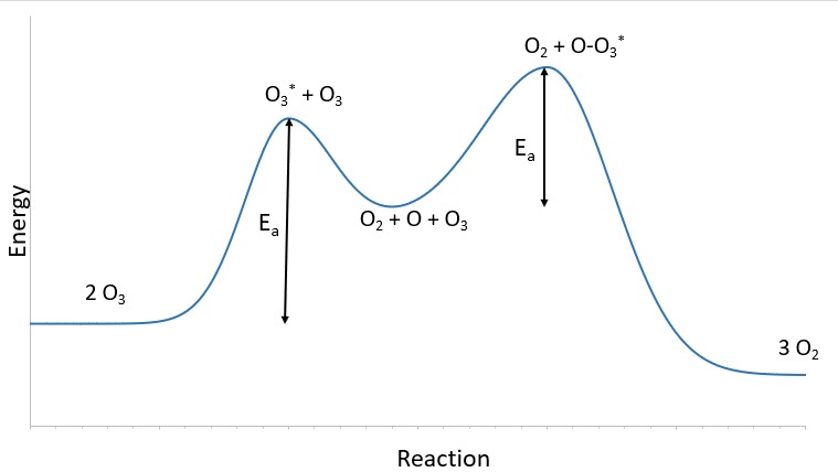
Notice that the oxygen atom produced in the first step of this mechanism is consumed in the second step and therefore does not appear as a product in the overall reaction. Species that are produced in one step and consumed in a subsequent step are called intermediates. Intermediates are different from transition states because the intermediates are longer lived and can be detected in many reactions. A transition state is at the top of the reaction energy diagram - as shown in Figure $\PageIndex{2}$. Figure $\PageIndex{4}$ shows the O₃ starting material, the first transition state is the excited state ozone molecule, O₃^*, the reaction intermediate O in the valley between the two transition state peaks, the second transition state O-O₃^*, and the final products O₂. T

activation energy diagram for ozone decomposition — Figure $\PageIndex{4}$:Energy diagram for ozone decomposition.

While the overall reaction equation for the decomposition of ozone indicates that two molecules of ozone react to give three molecules of oxygen, the mechanism of the reaction does not involve the direct collision and reaction of two ozone molecules. Instead, one O₃ decomposes to yield O₂ and an oxygen atom, and a second O₃ molecule subsequently reacts with the oxygen atom to yield two additional O₂ molecules.

Unlike balanced equations representing an overall reaction, the equations for elementary reactions are explicit representations of the chemical change taking place. The reactant(s) in an elementary reaction’s equation undergo only the bond-breaking and/or making events depicted to yield the product(s).

Unimolecular Elementary Reactions

The molecularity of an elementary reaction is the number of reactant species (atoms, molecules, or ions). For example, a unimolecular reaction involves the reaction of a single reactant species to produce one or more molecules of product:

$ \mathrm{A} \longrightarrow \mathrm{products} $

The rate law for a unimolecular reaction is first order because it only depends upon the amount of one reaction:

rate = k [A]

A unimolecular reaction may be one of several elementary reactions in a complex mechanism. For example, the reaction:

O₃ (g) -> O₂ (g) + O

illustrates a unimolecular elementary reaction that occurs as one part of a two-step reaction mechanism as described above. However, in some cases the overall reaction is also an elementary reaction. For some unimolecular reactions are the only step of a single-step reaction mechanism. For example, the gas-phase decomposition of cyclobutane, C₄H₈, to ethylene, C₂H₄, is represented by the chemical equation in Figure $\PageIndex{4}$:

Figure $\PageIndex{5}$. Decomposition of cyclobutane.

This equation represents the overall reaction observed, and it might also represent a legitimate unimolecular elementary reaction. The rate law predicted from this equation, assuming it is an elementary reaction, turns out to be the same as the rate law derived experimentally for the overall reaction, namely, one showing first-order behavior:

rate = k[C₄H₈]

This agreement between observed and predicted rate laws is interpreted to mean that the proposed unimolecular, single-step process is a reasonable mechanism for the butadiene reaction.

Bimolecular Elementary Reactions

A bimolecular reaction involves two reactant species, for example:

$ \mathrm{A}+\mathrm{A} \longrightarrow \mathrm{products} $

$ \mathrm{A}+\mathrm{B} \longrightarrow \mathrm{products} $

For the first type, in which the two reactant molecules are different, the rate law is first-order in A and first order in B (second-order overall):

$ \mathrm{RATE}= \mathrm{k[A][B]} $

For the second type, in which two identical molecules collide and react, the rate law is second order in A:

$ \mathrm{RATE}=\mathrm{k[A][A]}=\mathrm{k[A]^2} $

Some chemical reactions occur by mechanisms that consist of a single bimolecular elementary reaction. One example is the reaction of nitrogen dioxide with carbon monoxide shown in Figure $\PageIndex{6}$:

NO₂(g) + CO(g) ⟶ NO(g) + CO₂(g)

This figure provides an illustration of a reaction between two H I molecules using space filling models. H atoms are shown as white spheres, and I atoms are shown as purple spheres. On the left, two H I molecules are shownwith a small white sphere bonded to a much larger purple sphere. The label, “Two H I molecules,” appears below. An arrow points right to a similar structure in which the two molecules appear pushed together, so that the purple spheres of the two molecules are touching. Below appears the label, “Transition state.” Following another arrow, two white spheres are shown vertically oriented and bonded together with the label, “H subscript 2” above. The H subscript 2 molecule is followed by a plus sign and two purple spheres bonded together with the label, “I subscript 2” above. Below these structures is the label, “Hydrogen iodide molecules decompose to produce hydrogen H subscript 2 and iodine I subscript 2.”

Figure $\PageIndex{6}$ The probable mechanism for the reaction between NO₂ and CO to yield NO and CO₂.

Bimolecular elementary reactions may also be involved as steps in a multistep reaction mechanism. The reaction of atomic oxygen with ozone is the second step of the two-step ozone decomposition mechanism discussed earlier in this section.

Relating Reaction Mechanisms to Rate Laws

It’s often the case that one step in a multistep reaction mechanism has a much higher activation energy, so it is significantly slower than the others. Because a reaction cannot proceed faster than its slowest step, this step will limit the rate at which the overall reaction occurs. The slowest step is therefore called the rate-limiting step (or rate-determining step) of the reaction. Figure $\PageIndex{7}$ shows a cattle chute, which is the rate-determining step for moving cattle between two pens.

A photo is shown of cattle passing through a narrow chute into a holding pen. A person directs them through the gate with a long white and red pole.

Figure $\PageIndex{7}$ A cattle chute is a nonchemical example of a rate-determining step. Cattle can only be moved from one holding pen to another as quickly as one animal can make its way through the chute. (credit: Loren Kerns)

As described earlier, rate laws may be derived directly from the chemical equations for elementary reactions. However, most chemical reactions are not elementary reactions so and they are often the result of several elementary reaction steps. Together these steps make up the reaction mechanism. In every case, the rate law must be determined from experimental data and the reaction mechanism subsequently deduced from the rate law (and sometimes from other data). The reaction of NO₂ and CO provides an illustrative example:

NO₂(g)+CO(g)⟶CO₂(g)+NO(g)

For temperatures above 225 °C, the rate law is:

rate = k [NO₂][CO]

The reaction is first order with respect to NO₂ and first-order with respect to CO. This is consistent with a single-step bimolecular mechanism and it is possible that this is the mechanism for this reaction at high temperatures.

At temperatures below 225 °C, the reaction is described by a rate law that is second order with respect to NO₂:

rate=k[NO₂]²

This rate law is not consistent with the single-step mechanism, but is consistent with the following two-step mechanism:

NO₂(g)+NO₂(g)⟶NO₃(g)+NO(g) (slow)
NO₃(g)+CO(g)⟶NO₂(g)+CO₂(g) (fast)

The rate-determining (slower) step gives a rate law showing second-order dependence on the NO₂ concentration, and the sum of the two equations gives the net overall reaction. This shows the reaction using different mechanisms depending upon the temperature. The two reaction mechanisms are shown in Figure $\PageIndex{8}$.

Figure $\PageIndex{8}$: Copy and Paste Caption here. (Copyright; author via source)

In general, when the rate-determining (slower) step is the first step in a mechanism, the rate law for the overall reaction is the same as the rate law for this step. However, when the rate-determining step is preceded by a step involving a rapidly reversible reaction the rate law for the overall reaction may be more difficult to derive.

Search

Text Color

Text Size

Margin Size

Font Type