
4.2b: Differential Rate Law Snow Day
- Page ID
- 369432
\( \newcommand{\vecs}[1]{\overset { \scriptstyle \rightharpoonup} {\mathbf{#1}} } \)
\( \newcommand{\vecd}[1]{\overset{-\!-\!\rightharpoonup}{\vphantom{a}\smash {#1}}} \)
\( \newcommand{\id}{\mathrm{id}}\) \( \newcommand{\Span}{\mathrm{span}}\)
( \newcommand{\kernel}{\mathrm{null}\,}\) \( \newcommand{\range}{\mathrm{range}\,}\)
\( \newcommand{\RealPart}{\mathrm{Re}}\) \( \newcommand{\ImaginaryPart}{\mathrm{Im}}\)
\( \newcommand{\Argument}{\mathrm{Arg}}\) \( \newcommand{\norm}[1]{\| #1 \|}\)
\( \newcommand{\inner}[2]{\langle #1, #2 \rangle}\)
\( \newcommand{\Span}{\mathrm{span}}\)
\( \newcommand{\id}{\mathrm{id}}\)
\( \newcommand{\Span}{\mathrm{span}}\)
\( \newcommand{\kernel}{\mathrm{null}\,}\)
\( \newcommand{\range}{\mathrm{range}\,}\)
\( \newcommand{\RealPart}{\mathrm{Re}}\)
\( \newcommand{\ImaginaryPart}{\mathrm{Im}}\)
\( \newcommand{\Argument}{\mathrm{Arg}}\)
\( \newcommand{\norm}[1]{\| #1 \|}\)
\( \newcommand{\inner}[2]{\langle #1, #2 \rangle}\)
\( \newcommand{\Span}{\mathrm{span}}\) \( \newcommand{\AA}{\unicode[.8,0]{x212B}}\)
\( \newcommand{\vectorA}[1]{\vec{#1}} % arrow\)
\( \newcommand{\vectorAt}[1]{\vec{\text{#1}}} % arrow\)
\( \newcommand{\vectorB}[1]{\overset { \scriptstyle \rightharpoonup} {\mathbf{#1}} } \)
\( \newcommand{\vectorC}[1]{\textbf{#1}} \)
\( \newcommand{\vectorD}[1]{\overrightarrow{#1}} \)
\( \newcommand{\vectorDt}[1]{\overrightarrow{\text{#1}}} \)
\( \newcommand{\vectE}[1]{\overset{-\!-\!\rightharpoonup}{\vphantom{a}\smash{\mathbf {#1}}}} \)
\( \newcommand{\vecs}[1]{\overset { \scriptstyle \rightharpoonup} {\mathbf{#1}} } \)
\( \newcommand{\vecd}[1]{\overset{-\!-\!\rightharpoonup}{\vphantom{a}\smash {#1}}} \)
\(\newcommand{\avec}{\mathbf a}\) \(\newcommand{\bvec}{\mathbf b}\) \(\newcommand{\cvec}{\mathbf c}\) \(\newcommand{\dvec}{\mathbf d}\) \(\newcommand{\dtil}{\widetilde{\mathbf d}}\) \(\newcommand{\evec}{\mathbf e}\) \(\newcommand{\fvec}{\mathbf f}\) \(\newcommand{\nvec}{\mathbf n}\) \(\newcommand{\pvec}{\mathbf p}\) \(\newcommand{\qvec}{\mathbf q}\) \(\newcommand{\svec}{\mathbf s}\) \(\newcommand{\tvec}{\mathbf t}\) \(\newcommand{\uvec}{\mathbf u}\) \(\newcommand{\vvec}{\mathbf v}\) \(\newcommand{\wvec}{\mathbf w}\) \(\newcommand{\xvec}{\mathbf x}\) \(\newcommand{\yvec}{\mathbf y}\) \(\newcommand{\zvec}{\mathbf z}\) \(\newcommand{\rvec}{\mathbf r}\) \(\newcommand{\mvec}{\mathbf m}\) \(\newcommand{\zerovec}{\mathbf 0}\) \(\newcommand{\onevec}{\mathbf 1}\) \(\newcommand{\real}{\mathbb R}\) \(\newcommand{\twovec}[2]{\left[\begin{array}{r}#1 \\ #2 \end{array}\right]}\) \(\newcommand{\ctwovec}[2]{\left[\begin{array}{c}#1 \\ #2 \end{array}\right]}\) \(\newcommand{\threevec}[3]{\left[\begin{array}{r}#1 \\ #2 \\ #3 \end{array}\right]}\) \(\newcommand{\cthreevec}[3]{\left[\begin{array}{c}#1 \\ #2 \\ #3 \end{array}\right]}\) \(\newcommand{\fourvec}[4]{\left[\begin{array}{r}#1 \\ #2 \\ #3 \\ #4 \end{array}\right]}\) \(\newcommand{\cfourvec}[4]{\left[\begin{array}{c}#1 \\ #2 \\ #3 \\ #4 \end{array}\right]}\) \(\newcommand{\fivevec}[5]{\left[\begin{array}{r}#1 \\ #2 \\ #3 \\ #4 \\ #5 \\ \end{array}\right]}\) \(\newcommand{\cfivevec}[5]{\left[\begin{array}{c}#1 \\ #2 \\ #3 \\ #4 \\ #5 \\ \end{array}\right]}\) \(\newcommand{\mattwo}[4]{\left[\begin{array}{rr}#1 \amp #2 \\ #3 \amp #4 \\ \end{array}\right]}\) \(\newcommand{\laspan}[1]{\text{Span}\{#1\}}\) \(\newcommand{\bcal}{\cal B}\) \(\newcommand{\ccal}{\cal C}\) \(\newcommand{\scal}{\cal S}\) \(\newcommand{\wcal}{\cal W}\) \(\newcommand{\ecal}{\cal E}\) \(\newcommand{\coords}[2]{\left\{#1\right\}_{#2}}\) \(\newcommand{\gray}[1]{\color{gray}{#1}}\) \(\newcommand{\lgray}[1]{\color{lightgray}{#1}}\) \(\newcommand{\rank}{\operatorname{rank}}\) \(\newcommand{\row}{\text{Row}}\) \(\newcommand{\col}{\text{Col}}\) \(\renewcommand{\row}{\text{Row}}\) \(\newcommand{\nul}{\text{Nul}}\) \(\newcommand{\var}{\text{Var}}\) \(\newcommand{\corr}{\text{corr}}\) \(\newcommand{\len}[1]{\left|#1\right|}\) \(\newcommand{\bbar}{\overline{\bvec}}\) \(\newcommand{\bhat}{\widehat{\bvec}}\) \(\newcommand{\bperp}{\bvec^\perp}\) \(\newcommand{\xhat}{\widehat{\xvec}}\) \(\newcommand{\vhat}{\widehat{\vvec}}\) \(\newcommand{\uhat}{\widehat{\uvec}}\) \(\newcommand{\what}{\widehat{\wvec}}\) \(\newcommand{\Sighat}{\widehat{\Sigma}}\) \(\newcommand{\lt}{<}\) \(\newcommand{\gt}{>}\) \(\newcommand{\amp}{&}\) \(\definecolor{fillinmathshade}{gray}{0.9}\)
Ancillary Documents
UALR Students Use Documents in Google Classroom The following links allow anyone to make their own copy of the assignment, which they can modify and reuse, but students must use the copies provided in Google Classroom for grading.
- Copy of Worksheet I: Kinetics (Group Activity)
- Lab Report Page: Includes procedures, class data sheet, and Lab Report Template
Learning Objectives
Students will be able to:
Content
- Design a series experiments to calculate the constants involved in function, the rate law, where the value of the dependent variable (Rate Law) depends on three independent variables (concentration of two reactions and temperature).
- Apply this to the reaction of the reduction of Ferric Iron by Iodide at various temperatures.
- Understand how the initial rate of a chemical reaction producing iodine can be measured in an iodine clock reaction.
- Work up the data and calculate the rate constant at room temperature, the order of reaction with respect to Ferric and Iodide ions and the Arrhenius constant from rate law data.
- Understand the mathematics of all the calculations
Process
- Run experiments to measure the initial rate of reaction by varying three independant variables, [Fe+2], [I-] and T.
- Use a spreadsheet to calculate the order of reaction from log log plots of Rate and concentration data.
- Use a spreadsheet to calculate the Arrhenius constant from temperature and ln rate constant data.
- Report results
Prior Knowledge
- Redox Reactions (LibreText Section 3.6)
- Use of Logarithms (LibreText Section 14.0.2)
- Use of spreadsheets on log and natural log plots (Graphing Lab)
- Use of spreadsheet functions (Graphing Lab)
Recommended Prior Reading
Worksheet II: The Experiment
The second part of the lab will go over running the experiment and working up the data. Do to winter weather you will not be able to mix actual reagents but we will go over the procedures and you are responsible for understanding basic laboratory techniques like reading a burette, along with safe operating procedures like wearing safety glasses. In the real lab students would work in groups of two, mix the solutions and record the time it takes for the solution to turn blue. There is an element of error intrinsic error in the data of this lab, as for example, we are basing the reaction time on a subjective observation, when a solution turns blue. That is, two students who are looking at the exact same reaction might record different times because they interpret different shades of blue to indicate the reaction is over. Likewise, inconsistent mixing could induce error both within experiments of a group, and across groups. If these errors are random in contrast to systematic (see section 1B.2), the effects can be minimized by running lots of experiments, and so the class would all share their data. So we will watch three videos, one of each experiment and record the time to turn blue, and then add that data to a data set created by a previous class, and then like the previous class, work up the entire data set (including the values we contributed with our observations of the videos).
There are two approaches to working up large sets of data, convert the measured values to average values and plot that, or use spreadsheets to calculate the multiple values and then plot all of the data. In lab 2 we were introduced to the use of equations on Google Sheets, and in this lab we will build a Workbook in Google Sheets where we not only work up all the data, but create a dashboard on the front page of the workbook and then create a separate sheet within the workbook for each of the three experiments we ran, showing all calculations involved in each graph. Therefore, in addition to Worksheet II students will need to develop and submit a workbook in Google Sheets and unlike the first worksheet, this is an individual assignment where each student submits an individual worksheet and workbook, although students are encouraged to work these up as teams, but each student needs to submit their own workbook and worksheet for grading.
Part V: Obtaining the Data
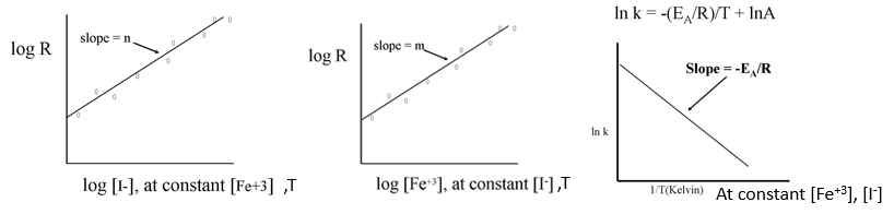
In part IV you designed the three experiments needed to run to obtain the constants (m, n and EA). The following table shows 5 experimental conditions where 50 mL of the two reagents were mixed and the time was recorded until the solution turned blue. Students work in groups and share their data. Each experiment is identified by an experiment number (1-5) and table \(\PageIndex{1}\) shows the concentrations and volumes of reagents mixed. Students will work this data up with three graphs.
- Graph 1: Experiments 1-3: Order of rxn with respect to [Fe+3 ] at T3 = room, [I-]= constant.
- Graph 2: Experiments 3-5: Order of rxn with respect to [I-] at T3 = room, [Fe+3] = constant
- Graph 3: Experiment 3: Arrhenius constant, at different T3 , with [Fe+3] and [I-] held constant
|
Reagent 1 250 mL Erlenmeyer Flask |
Reagent 2 100 mL Beaker |
After Mixing | ||||||||
| Exp. # |
0.04M |
0.15M |
H2O |
Exp. # |
0.04M |
0.004M S2O3-2 |
Starch, (mL) |
H2O, (mL) |
Temp |
|
| 1 | 20.00 | 20.00 | 10.00 | 1 | 10.00 | 10.00 |
5.00 |
25.00 | room | |
| 2 | 15.00 | 20.00 | 15.00 | 2 | 10.00 | 10.00 |
5.00 |
25.00 | room | |
| 3 | 10.00 | 20.00 | 20.00 | 3 | 10.00 | 10.00 |
5.00 |
20.00 |
room or variable |
|
| 4 | 10.00 | 20.00 | 15.00 | 4 | 15.00 | 10.00 |
5.00 |
15.00 | room | |
| 5 | 10.00 | 20.00 | 10.00 | 5 | 20.00 | 10.00 |
5.00 |
15.00 | room | |
Table 1: volumes and concentrations of solutions mixed in the different experimental runs
You goal is to calculate the Rate at t=0 (moment of mixing) as the reaction starts the moment the two solutions are mixed. If both of the above flasks have 50 mL the total of the combined solution will be 100 mL. To calculate the concentration of any reagent at the moment of mixing you use the dilution equation, please review section 4.4.3
\[M_iV_i=M_fV_f\]
Where Mi is the initial Molarity (added to either reagent flask), Vi is the initial volume (added to either reagent flask), Mf is the final molarity (in the reaction flask) and Vf is the final volume of the mixture (100 ml). So
\[M_f=M_i \frac{V_i}{V_f}\]
note, the term \(\frac{V_i}{V_f}\) is often called the dilution factor, and is dimensionless if both volumes have the same units.
These concentrations need to be calculated for both reactants ([Fe+3] and [I-]) in each experiment along with the thiosulfate concentration ([S2O3-2]) that is used to calculate the initial rate. Figure 2 shows the table of the Google Doc where you post the ferric iron and iodide concentrations.
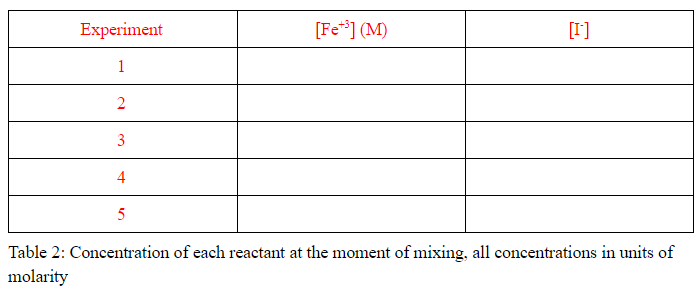
Figure \(\PageIndex{2}\): Screen capture of Google Worksheet table where they record values of ferric and iodide ions
Before proceeding complete activities 1 and 2 of the Google Doc associated with this activity if assigned
Part VI: The Data
The following table provides a experimental data that was pooled by a class. The trial number represents the number of times the students repeated an experiment and the experiment number is aligned with the concentrations used in table 2 of figure 2 (above). You should plot all the data in your google sheets workbook (not use average values) and experiment 3 room temperature data should be used in all three graphs.
| Trial # | Exp. # | Time (s) | Temp (oC) | Group # | Exp. # | Time (s) | Temp (oC) | |
| 1 | 1 | 29.45 | 22.90 | 2 | 4 | 75.03 | 22.90 | |
| 2 | 1 | 32.36 | 22.90 | 3 | 4 | 77.78 | 22.90 | |
| 3 | 1 | 29.88 | 22.90 | 4 | 4 | 67.82 | 22.90 | |
| 4 | 1 | 29.32 | 22.90 | 5 | 4 | 79.97 | 22.90 | |
| Video | 1 | 22.90 | 6 | 4 | 67.56 | 22.90 | ||
| 1 | 2 | 52.03 | 22.90 | Video | 4 | 22.90 | ||
| 2 | 2 | 54.69 | 22.90 | 1 | 5 | 52.90 | 22.90 | |
| 3 | 2 | 52.60 | 22.90 | 2 | 5 | 55.10 | 22.90 | |
| 4 | 2 | 55.29 | 22.90 | 3 | 5 | 66.44 | 22.90 | |
| 5 | 2 | 56.50 | 22.90 | 4 | 5 | 65.90 | 22.90 | |
| 6 | 2 | 50.00 | 22.90 | 5 | 5 | 57.10 | 22.90 | |
| 7 | 2 | 52.60 | 22.90 | 6 | 5 | 53.29 | 22.90 | |
| Video | 2 | 22.90 | Video | 5 | 22.90 | |||
| 1 | 3 | 120.01 | 22.90 | 1 | 3, TCold | 254.85 | 16.30 | |
| 2 | 3 | 121.12 | 22.90 | 2 | 3, TCold | 265.52 | 19.90 | |
| 3 | 3 | 126.33 | 22.90 | 3 | 3, TCold | 242.79 | 17.30 | |
| 4 | 3 | 129.56 | 22.90 | 4 | 3, TCold | 438.20 | 14.20 | |
| 5 | 3 | 118.14 | 22.90 | Video | 3, TCold | 21.40 | ||
| 6 | 3 | 125.69 | 22.90 | 1 | 3, THot | 13.55 | 35.30 | |
| 7 | 3 | 128.55 | 22.90 | 2 | 3, THot | 20.97 | 35.80 | |
| Video | 3 | 22.90 | 3 | 3, THot | 20.32 | 34.90 | ||
| 1 | 4 | 72.59 | 22.90 | Video | 3, THot | 25.01 | ||
| Video | 3, THot | 30.67 |
The following videos were taken of various solutions and you need to watch them and insert into the spreadsheet the missing data
|
Video \(\PageIndex{5}\): Iodine Clock Experiment 1 (V.S. Belford) |
[Fe+3] = 0.008M |
Video \(\PageIndex{4}\): Iodine Clock Experiment 2 (V.S. Belford) https://youtu.be/OCzPDUk6Tks |
[Fe+3] = 0.006M |
| [ I-] = 0.004M | [ I-] = 0.004M | ||
| [S2O3-2] = 0.0004M | [S2O3-2] = 0.0004M | ||
| T = 22.90 ℃ | T = 22.90 ℃ |
|
Video \(\PageIndex{3}\): Iodine Clock Experiment 3 (V.S. Belford) |
[Fe+3] = 0.004M |
Video \(\PageIndex{2}\): Iodine Clock Experiment 4 (V.S. Belford) https://youtu.be/ZaudifbeKwg |
[Fe+3] = 0.004M |
| [ I-] = 0.004M | [ I-] = 0.006M | ||
| [S2O3-2] = 0.0004M | [S2O3-2] = 0.0004M | ||
| T = 22.90 ℃ | T = 22.90 ℃ |
|
Video \(\PageIndex{1}\): Iodine Clock Experiment 5 (V.S. Belford) https://youtu.be/M1JpDpBuTUM |
[Fe+3] = 0.004M |
Video \(\PageIndex{6}\): Iodine Clock Experiment 3 at T=21.40 ℃ (V.S. Belford) https://youtu.be/OCzPDUk6Tks |
[Fe+3] = 0.004M |
| [ I-] = 0.008M | [ I-] = 0.004M | ||
| [S2O3-2] = 0.0004M | [S2O3-2] = 0.0004M | ||
| T = 22.90 ℃ | T = 21.40 ℃ |
|
Video \(\PageIndex{1}\): Iodine Clock Experiment at T=25.01 ℃ (V.S. Belford) https://youtu.be/6jHEFzBGL8o |
[Fe+3] = 0.004M |
Video \(\PageIndex{2}\): Iodine Clock Experiment at T=30.67 (V.S. Belford) https://youtu.be/OCzPDUk6Tks |
[Fe+3] = 0.004M |
| [ I-] = 0.004M | [ I-] = 0.004M | ||
| [S2O3-2] = 0.0004M | [S2O3-2] = 0.0004M | ||
| T = 25.01℃ | T = 30.67 ℃ |
The Failed Experiment
In this video a student forgot a reagent, can you figure out which one?
- Answer
-
Thiosulfate, the reaction instantly turns blue as there is no thiosulfate to stop iodine from accumulating.
Part VII: Working up the Data and Google Sheets Workbooks
There are three graphs we need to plot, the first two deal with the power function relationships of the constant temperature rate law (eq. 4.2) and the third deals with the temperature dependence of the rate constant (eq. 4.3)
Use the regular Lab Page