1.5: X-rays and X-ray Diffraction

HISTORICAL INTRODUCTION

X-rays were discovered during the summer of 1895 by Wilhelm Röntgen at the University of Würtzburg (Germany). Röntgen was interested in the cathode rays (beams of electrons) developed in discharge tubes, but it is not clear exactly which aspects of cathode rays he intended to study. By chance he noticed that a fluorescent screen \(\left(\mathrm{ZnS}+\mathrm{Mn}^{++}\right)\) lying on a table some distance from the discharge tube emitted a flash of light each time an electrical discharge was passed through the tube. Realizing that he had come upon something completely new, he devoted his energies to investigating the properties of the unknown ray " \(X\) " which produced this effect. The announcement of this discovery appeared in December 1895 as a concise ten page publication.

The announcement of the discovery of X-rays was received with great interest by the public. Röntgen himself prepared the first photographs of the bones in a living hand, and use of the radiation was quickly adopted in medicine. In the succeeding fifteen years, however, very few fundamental insights were gained into the nature of X-radiation. There was some indication that the rays were waves, but the evidence was not clear-cut and could be interpreted in several ways. Then, at the University of Munich in 1912, Max von Laue performed one of the most significant experiments of modern physics. At his suggestion, Paul Knipping (who had just completed a doctoral thesis with Röntgen) and Walter Friedrich (a newly appointed assistant to Sommerfeld) directed a beam of X-rays at a crystal of copper sulfate and attempted to record the scattered beams on a photographic plate. The first experiment was unsuccessful. The result of a second experiment was successful. They observed the presence of spots produced by diffracted X-ray beams grouped around a larger central spot where the incident X-ray beam struck the film. This experiment demonstrated conclusively that X-radiation consisted of waves and, further, that the crystals were composed of atoms arranged on a space lattice.

ORIGIN OF X-RAY SPECTRA

The interpretation of X–ray spectra according to the Bohr theory (LN-1) of electronic levels was first (and correctly) proposed by W. Kossel in 1920: the electrons in an atom are arranged in shells (K, L, M, N, corresponding to n = 1, 2, 3, 4, ..., etc.). Theory predicts that the energy differences between successive shells increase with decreasing n and that the electron transition from n = 2 to n = 1 results in the emission of very energetic (short wavelength) radiation (fig. 1), while outer shell transitions (say, from \(n=5\) to \(n=4\) ) yield low energy radiation (long wavelength). For hydrogen, you recall, the wave number of the emitted radiation associated with a particular electron transition is given by the Rydberg equation:

\(\bar{v}=\left(\dfrac{1}{n_i^2}-\dfrac{1}{n_f^2}\right) R\)

For "hydrogen-like" atoms with the atomic number \(Z\) (containing one electron only) the corresponding Rydberg equation becomes:

\(\bar{v}=\left(\dfrac{1}{n_i^2}-\dfrac{1}{n_f^2}\right) R Z^2\)

From this relationship it is apparent that the energy difference associated with electron transitions increases strongly with the atomic number and that the wavelength of radiation emitted during such transitions moves with increasing \(Z\) from the \(10^{-7} \mathrm{~m}\) range to the \(10^{-10} \mathrm{~m}\) range (radiation now defined as \(\mathrm{X}\)-rays).

Figure 1 X-rays are generated by inner shell electron transitions

To bring about such inner shell transitions requires the generation of an electron vacancy: an electron must be removed, for example from the \(\mathrm{K}\) shell \((\mathrm{n}=1)\), of an atom. Such a vacancy is conveniently produced in an X-ray tube by an electron beam (generated by a heated filament which is made a cathode) impinging, after being subjected to an accelerating potential of several \(\mathrm{kV}\), into a target material made anode (fig. 2). The impinging electrons will transfer part of their energy to electrons of the target material and result in electronic excitation. If the energy of the arriving electrons is high enough, some may knock out a \(\mathrm{K}\) shell electron in the target and thus generate a vacancy. [It should be clear that a \(\mathrm{K} \rightarrow \mathrm{L}\) excitation cannot take place since the \(\mathrm{L}\) shell is filled: excitation must involve \((n=1) \rightarrow(n=\infty)\).] When such a vacancy is generated, it can readily be filled by an electron from the \(L\) shell or the \(M\) shell of the same atom. These internal electron transitions give rise to the emission of "characteristic" X-radiation which, because of its short wavelength, has extremely high "penetrating" power.

Since an electron beam is used to generate \(X\)-rays, the \(X\)-ray tube has to be evacuated: to dissipate the energy flux arriving at the target, the anode support (onto which the target is mounted) is water-cooled.

Figure 2 Generation of x-rays

Under standard operating conditions, the characteristic radiation emitted by the target comprises two sharp lines, referred to as \(\mathrm{K}_\alpha\) and \(\mathrm{K}_\beta\) lines (fig. 3). They are associated, respectively, with electron transitions from \(n=2\) to \(n=1\) and from \(n=3\) to \(n=1\).

Emitted X-ray spectra were extensively studied by H.G.J. Moseley who established the relationship between the wavelength of characteristic radiation and the atomic number \(\mathrm{Z}\) of the radiation emitting target material (fig. 4). Experimentally he found that the \(\mathrm{K}_\alpha\) lines for various target materials (elements) exhibit the relationship:

\(\lambda K_\alpha \propto \dfrac{1}{Z^2} \quad\left(\bar{v} K_\alpha \propto Z^2\right)\)

Moseley’s empirical relationship (which reflects a behavior in agreement with the Rydberg equation) can be quantified. While the energy levels associated with outer electron transitions are significantly affected by the “screening” effect of inner electrons (which is variable and cannot as yet be determined from first principles), the conditions associated with X-ray generation are simple. Very generally, the screening effect of the innermost electrons on the nuclear charge is accounted for in an effective nuclear charge \((Z-\sigma)\) and the Rydberg equation assumes the form:

\(\bar{v}=\left(\dfrac{1}{n_i^2}-\dfrac{1}{n_f^2}\right) R(Z-\sigma)^2\)

where \(\sigma=\) screening effect

Figure 4 Moseley relationship for \(\mathrm{K}_{\alpha}\) and \(\mathrm{L}_{\alpha}\) radiation

Considering the transition \(n_2 \rightarrow n_1\), screening of the full nuclear charge is only provided by the one electron remaining in the K shell. Thus it is possible to use the ν modified Rydberg equation, taking \(\sigma = 1\). Accordingly, we have:

\(\bar{v} K_\alpha=\left(\dfrac{1}{2^2}-\dfrac{1}{1^2}\right) R(Z-1)^2=-\dfrac{3}{4} R(Z-1)^2\)

where: \(\mathrm{R}=\) Rydberg constant and \(\mathrm{Z}=\) atomic number of the target material. [The minus sign (-) only reflects radiative energy given off by the system.]

Figure 3 Electronic transitions giving rise to characteristic X- ray spectra.

Similarly, for the characteristic \(L_\alpha\) series of spectral lines ( \(n=3\) to \(n=2\) ) we find, after removal of one \(\mathrm{L}\) electron, that the screening of the electrons in the \(\mathrm{K}\) shell and the remaining electrons in the \(L\) shell reduces the nuclear charge by 7.4 (empirical value).

\(\overline{\mathrm{v}} \mathrm{L}_\alpha=\left(\dfrac{1}{3^2}-\dfrac{1}{2^2}\right) \mathrm{R}(\mathrm{Z}-7.4)^2=-\dfrac{5}{36} \mathrm{R}(\mathrm{Z}-7.4)^2\)

A second look at the X-ray spectrum of a Mo target, obtained with an electron accelerating potential of \(35 \mathrm{kV}\) (fig. 5), shows that the characteristic radiation \(\left(\mathrm{K}_\alpha, \mathrm{K}_\beta\right)\) appears superimposed on a continuous spectrum (continuously varying \(\lambda\) ) of lower and varying intensity. This continuous spectrum is referred to as bremsstrahlung (braking radiation) and has the following origin. Electrons, impinging on the target material, may lose their energy by transferring it to orbiting electrons, as discussed above; in many instances, however, the electrons may come into the proximity of the force fields of target nuclei and, in doing so, will be "slowed down" or decelerated to a varying degree,

Figure 5 X-ray spectrum of Mo target as a function of applied Voltage.

ranging from imperceptible deceleration to total arrest. The energy lost in this slowing down process is emitted in the form of radiation (braking radiation, or bremsstrahlung). This energy conversion, as indicated, can range from partial to complete (fig. 6). The

Figure 6 Origin of Bremsstrahlung; the continuous part of the X-ray spectrum

incident electrons have an energy of \(\mathrm{e} \cdot \mathrm{V}\) (electronic charge times accelerating Voltage) in the form of kinetic energy \(\left(\mathrm{mv}^2 / 2\right)\), and their total energy conversion gives rise to a Shortest Wavelength \((S W L)\) - the cut-off of the continuous spectrum for decreasing values of \(\lambda\) (fig. 5). Analytically, we have:

\(\mathrm{eV}=\mathrm{h} v_{\max }=\mathrm{h} \dfrac{\mathrm{c}}{\lambda_{\mathrm{SWL}}} \quad ; \quad \lambda_{\mathrm{SWL}}=\frac{\mathrm{hc}}{\mathrm{eV}}\)

From this relationship it is evident that the cut-off of the continuous spectrum toward decreasing \(\lambda^{\prime}\)'s \(\left(\lambda_{\mathrm{SWL}}\right)\) is controlled by the accelerating potential (fig. 5).

“FINE STRUCTURE” OF CHARACTERISTIC X-RAYS

It is customary to consider the characteristic \(\mathrm{X}\)-ray spectral lines as discrete lines \(\left(\mathrm{K}_\alpha\right.\), \(K_\beta, L_\alpha, L_\beta\), etc.). In reality, they are not discrete since the electron shells involved in the associated electron transitions have energy sublevels (s, p, d orbitals). These sublevels give rise to a "fine structure" insofar as the \(\mathrm{K}_\alpha\) lines are doublets composed of \(\mathrm{K}_{\alpha 1}\) and \(\mathrm{K}_{\alpha 2}\) lines. Similarly, \(L_\alpha, L_\beta\), etc., exhibit a fine structure.

These considerations suggest that X-ray spectra contain information concerning the energetics of electronic states. Obviously, analysis of X-rays emitted from a target of unknown composition can be used for a quantitative chemical analysis. [This approach is taken routinely in advanced scanning electron microscopy (SEM) where X-rays, generated by the focused electron-beam, are analyzed in an appropriate spectrometer.]

In fundamental studies it is also of interest to analyze soft (long \(\lambda\) ) \(X\)-ray spectra. For example, take the generation of \(\mathrm{X}\)-rays in sodium ( \(\mathrm{Na})\). By generating an electron vacancy in the \(\mathrm{K}\) shell, a series of \(\mathrm{K}_\alpha\) and \(\mathrm{K}_\beta\) lines will result. The cascading electron generates vacancies in the \(2 p\) level, which in turn can be filled by electrons entering from the 3s level (generation of "soft" X-rays). If the X-rays are generated in a Na vapor, the \(3 s \rightarrow 2 p\) transition will yield a sharp line; on the other hand, if \(X\)-rays are analyzed in sodium metal, the same transition results in the emission of a continuous broad band, about \(30 \AA\) in width. This finding confirms the existence of an energy band (discussed earlier).

An analysis of the width and intensity distribution of the X-ray band provides experimental data concerning the energy band width and the energy state density distribution within the energy band (fig. 7).

Figure 7 Soft X-rays from 3s - 2p transitions in solid Na and Na vapor

X-RAYS FOR STRUCTURAL ANALYSIS

The extensive use of \(X\)-rays for the analysis of atomic structural arrangements is based on the fact that waves undergo a phenomenon called diffraction when interacting with systems (diffracting centers) which are spaced at distances of the same order of magnitude as the wavelength of the particular radiation considered. X-ray diffraction in crystalline solids takes place because the atomic spacings are in the \(10^{-10} \mathrm{~m}\) range, as are the wavelengths of \(\mathrm{X}\)-rays.

DIFFRACTION AND BRAGG’S LAW

The atomic structure of crystalline solids is commonly determined using one of several different X-ray diffraction techniques. Complementary structure information can also be obtained through electron and neutron diffraction. In all instances, the radiation used must have wavelengths in the range of \(0.1\) to \(10 \AA\) because the resolution (or smallest object separation distance) to which any radiation can yield useful information is about equal to the wavelength of the radiation, and the average distance between adjacent atoms in solids is about \(10^{-10} \mathrm{~m}(1 \AA)\). Since there is no convenient way to focus \(\mathrm{X}\)-rays with lenses and to magnify images, we do not attempt to look directly at atoms. Rather, we consider the interference effects of \(X\)-rays when scattered by the atoms, comprising a crystal lattice. This is analogous to studying the structure of an optical diffraction grating by examining the interference pattern produced when we shine visible light on the grating. (The spacing of lines on a grating is about 0.5 to 1 µm and the wavelength of visible radiation ranges from 0.4 to 0.8 µm.) In the optical grating the ruled lines act as scattering centers, whereas in a crystal it is the atoms (more correctly, the electrons about the atom) which scatter the incident radiation.

The geometrical conditions which must be satisfied for diffraction to occur in a crystal were first established by Bragg. He considered a monochromatic (single wavelength) beam of X-rays with coherent radiation (X-rays of common wave front) to be incident on a crystal, as shown in fig. 8. Moreover, he established that the atoms which

Figure 8 Bragg's law, assuming the planes of atoms behave as reflecting planes.

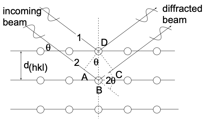
constitute the actual scattering centers can be represented by sets of parallel planes (in which the atoms are located) which act as mirrors and "reflect" the X-rays. In cubic systems the spacing of these planes, \(\mathrm{d}_{(\mathrm{hkl})}\) (see \(\left.\mathrm{LN}-4\right)\), is related to the lattice constant

(a):

\[\mathrm{d}_{(\mathrm{hkl})}=\dfrac{\mathrm{a}}{\sqrt{\mathrm{h}^2+\mathrm{k}^2+\mathrm{I}^2}} \tag{1}\]

For constructive interference of the scattered X-rays (the appearance of a diffraction peak) it is required that the beams, scattered on successive planes, be "in phase" (have again a common wave front) after they leave the surface of the crystal. In terms of the beams labeled 1 and 2 in fig. 8 this requires that the distance \(\overline{\mathrm{AB}}+\overline{\mathrm{BC}}\) be equal to an integral number of wavelengths \((\lambda)\) of the indicent radiation. Accordingly:

\(\overline{\mathrm{AB}}+\overline{\mathrm{BC}}=\mathrm{n} \lambda \quad(\mathrm{n}=1,2,3, \ldots)\)

Since \(\overline{\mathrm{AB}}=\overline{\mathrm{BC}}\) and \(\sin \theta=\frac{\overline{A B}}{d_{(h k)}}\left[\overline{A B}=d_{(h k)} \sin \theta\right]:\)

\[\mathrm{n} \lambda=2 \mathrm{~d}_{(\mathrm{hkl})} \sin \theta \tag{2}\]

This relation is referred to as Bragg's Law and describes the angular position of the diffracted beam in terms of \(\lambda\) and \(d_{(h k l)}\). In most instances of interest we deal with first order diffraction (\(n=1)\) and, accordingly, Bragg's law is:

\(\lambda=2 d_{(h k l)} \sin \theta\)

[We are able to make \(n=1\) because we can always interpret a diffraction peak for \(n=2,3, \ldots\) as diffraction from (nh \(n k n l)\) planes - i.e., from planes with one-nth the interplanar spacing of \(\left.d_{(\mathrm{hkl})} \cdot\right]\).

If we consider fig. 8 as representative for a "diffractometer" set-up (fig. 11), we have a collimated beam of X-rays impinging on a (100) set of planes and at \(2 \theta\) to the incident beam a detector which registers the intensity of radiation. For a glancing incident beam (small \(\theta)\) the detector will register only background radiation. As \(\theta\) increases to a value for which \(2 d \sin \theta=\lambda\), the detector will register high intensity radiation - we have a diffraction peak. From the above it is evident that the diffraction angle \((\theta)\) increases as the interplanar spacing, \(\mathrm{d}_{(\mathrm{hkl})}\), decreases.

The diffraction experiment as presently considered is intended to provide quantitative information on the volume (the lattice constant a) and shape characteristics (SC, BCC, FCC) of the unit cell. The intensity of diffraction peaks depends on the phase relationships between the radiation scattered by all the atoms in the unit cell. As a result, it happens quite often that the intensity of a particular peak, whose presence is predicted by Bragg's law, is zero. (This is because Bragg's law deals not with atom positions, but only with the size and shape of the unit cell.) For example, consider the intensity of the (100) diffraction peak of a crystal which has a BCC unit cell. The phase relationships show that the X-rays scattered at the top and bottom faces of the unit cell, (100) planes, interfere constructively, but are \(180^{\circ}\) out of phase with the X-rays scattered by the atom at the center of the unit cell. The resultant intensity is therefore zero. The rules which govern the presence of particular diffraction peaks in the different cubic Bravais lattices (SC, BCC and FCC) are given in Table I.

TABLE I. Selection Rules for Diffraction Peaks in Cubic Systems

\(\begin{array}{lcc}
\underline{\text { Bravais Lattice } }& \underline{\text { Reflections Present }} & \underline{\text { Reflections Absent }} \\
\text { Simple Cubic } & \text { All } & \text { None } \\ \\
\text { Body-Centered Cubic } & (\mathrm{h}+\mathrm{k}+\mathrm{l})=\text { even } & (\mathrm{h}+\mathrm{k}+\mathrm{l})=\text { odd } \\ \\
\text { Face-Centered Cubic } & \begin{array}{l}
\mathrm{h}, \mathrm{k}, \mathrm{l} \text { unmixed } \\
\text { (either all odd } \\
\text { or all even) }
\end{array} & \mathrm{h}, \mathrm{k}, \mathrm{l} \text { mixed } \\
& \begin{array}{c}
\end{array}
\end{array}\)

The rules given are strictly true only for unit cells where a single atom is associated with each lattice point. (Unit cells with more than one atom per lattice point may have their atoms arranged in positions such that reflections cancel. For example, diamond has an FCC Bravais lattice with two atoms per lattice point. All reflections present in diamond have unmixed indices, but reflections such as {200}, {222} and {420} are missing. The fact that all reflections present have unmixed indices indicates that the Bravais lattice is FCC – the extra missing reflections give additional information as to the exact atom arrangement.)

A hypothetical diffraction experiment: A material is known to be of simple cubic structure; determine a, the lattice constant, by X-ray diffraction. In theory, the question may be answered by placing the crystal into a diffractometer, rotating it into all possible positions relative to the incident \(X\)-ray beam and recording all diffracting \(2 \theta\) values. From the above we know that the smallest observed \(\theta\) value must correspond to diffraction on \(\{100\}\) planes and also that \(d_{(100)}=a\). We may now use Bragg's equation to determine a, the lattice constant:

\begin{aligned}
&\lambda=2 d \sin \theta=2 a \sin \theta \\
&a=\frac{\lambda}{2 \sin \theta}
\end{aligned}

There are two simplifying assumptions in this problem: (1) we know the system is SC and (2) we are able, through rotation, to bring all planes present into diffraction conditions.

EXPERIMENTAL APPROACHES TO X-RAY DIFFRACTION

In the context of this course we are interested in making use of X-ray diffraction for the purpose of (a) identifying (cubic) crystal systems, (b) determining the lattice constant, a, and (c) identifying particular planes or meaningful orientations. The possible approaches can, in principle, be identified through an examination of Bragg's law. The Bragg condition for particular \(\mathrm{d}_{(\mathrm{hkl})}\) values can be satisfied by adjusting either one of two experimental variables: (a) \(\lambda\), the wavelength of the X-ray beam used, or (b) \(\theta\), the orientation of the crystal planes relative to the incident X-rays.

(a) Fixed \(\theta\). Variable \(\lambda\): One means of satisfying Bragg's law is to irradiate a stationary single crystal ( \(\theta\) fixed for all planes within the crystal) with an X-ray beam of "white" radiation, which contains the characteristic and continuous spectrum produced by an X-ray tube. (For \(\lambda\) variable we have the simultaneous exposure of a crystal to a range of \(\lambda\) values). Each set of planes will reflect (diffract) the particular \(\lambda\) which satisfies the Bragg condition for the fixed \(\theta\). The diffracted beams may conveniently be recorded with a Polaroid camera or, alternately, with an electronic imaging device. It is possible to analyze either the transmitted or the back-reflected X-rays. This experimental procedure is referred to as the Laue technique (fig. 9); it is mostly conducted in the back-reflection mode. Note that the approach taken makes it possible to determine the values of \(\theta\) for each reflection, but not the corresponding \(\lambda\). Therefore, the technique cannot be used, for example, to determine lattice constants. However, it is very valuable if particular planes or crystal orientations are to be identified.

Figure 9: Laue diffraction in (a) transmission and (b) back-reflection mode.

Long

This is a figure with information about the process described in this section.

The figure has several sections of important information:

• This is the description of the first section.
• The middle section of the figure contains this information.
• The third and final section of the figure has this information.

(b)Fixed \(\lambda\) (Monochromatic X-Rays), Variable \(\theta\): The basic prerequisite for this approach is the availability of a monochromatic \(X\)-radiation of known wavelength \((\lambda)\). Such radiation can be conveniently obtained by using a crystal (i.e., its diffracting property) as a filter or monochromator (fig. 10). Filter action is achieved by positioning the crystal in such a way that the unfiltered radiation emitted by the X-ray tube becomes incident at an angle, \(\theta\), on a set of low index planes which satisfy Bragg's law for the highest intensity radiation \(\left(K_\alpha\right)\) emitted. The condition of a fixed \(\lambda\) and variable \(\theta\) is experimentally used in two techniques. Using a diffractometer (fig. 11), we place a sample (ground to a powder) into the center of a rotating stage and expose it to a monochromatic X-ray beam. The sample is rotated into diffraction condition and the diffraction angle determined.

Figure 10 Isolation of monochromatic radiation from target radiation

Figure 11 X-ray Diffractometer setup.

In the Debye-Scherrer method (fig.12) the sample is ground to a powder and placed (in an ampoule) into the center of a Debye-Scherrer camera. Exposed to monochromatic X-rays, in this way a large number of diffracted cone-shaped beams are generated such that the semiangles of the cones measure \(2\theta\), or twice the Bragg angle for the particular diffracting crystallographic planes. The reason diffracted beams are cone-shaped is that the planes in question (within the multitude of randomly oriented grains) give rise to diffraction for any orientation around the incident beam as long as the incident beam forms the appropriate Bragg angle with these planes – thus there is a rotational symmetry of the diffracted beams about the direction of the incident beam. Those planes with the largest interplanar spacing have the smallest Bragg angle, \(\theta\).

Figure 12 Debye-Scherrer powder diffraction setup and analysis

In a Debye-Scherrer arrangement, after exposing a powder of a crystalline material to monochromatic X-rays, the developed film strip will exhibit diffraction patterns such as indicated in fig. 12. Each diffraction peak (dark line) on the film strip corresponds to constructive interference at planes of a particular interplanar spacing \(\left[\mathrm{d}_{(\mathrm{hkl})}\right]\). The problem now consists of "indexing" the individual lines - i.e., determining the Miller indices (hkl) for the diffraction lines:

\begin{aligned}
\text { Bragg: } \quad \lambda &=2 \mathrm{~d}_{(\mathrm{hkl})} \sin \theta & ; & \mathrm{d}_{(\mathrm{hkl})} &=\frac{\mathrm{a}}{\sqrt{\mathrm{h}^2+\mathrm{k}^2+\mathrm{l}^2}} \\
\lambda^2 &=4 \mathrm{~d}_{(\mathrm{hkl})}^2 \sin ^2 \theta & ; & \mathrm{d}_{(\mathrm{hkl})}^2 &=\frac{\mathrm{a}^2}{\left(\mathrm{~h}^2+\mathrm{k}^2+\mathrm{l}^2\right)}
\end{aligned}

Substitution and rearrangement of above yields:

\(\dfrac{\sin ^2 \theta}{\left(h^2+k^2+\left.\right|^2\right)}=\dfrac{\lambda^2}{4 a^2}=\text { const. }\)

Accordingly, we find that for all lines (\(\theta\) values) of a given pattern, the relationship

\(\dfrac{\sin ^2 \theta_1}{\left(h^2+k^2+\left.\right|^2\right)_1}=\dfrac{\sin ^2 \theta_2}{\left(h^2+k^2+\mathrm{I}^2\right)_2}=\dfrac{\sin ^2 \theta_3}{\left(h^2+k^2+\mathrm{I}^2\right)_3}=\text { const. }\)

holds. Since the sum \(\left(h^2+k^2+l^2\right)\) is always integral and \(\lambda^2 / 4 a^2\) is a constant, the problem of indexing the pattern of a cubic system is one of finding a set of integers \(\left(h^2+k^2+l^2\right)\) which will yield a constant quotient when divided one by one into the observed \(\sin ^2 \theta\) values. (Certain integers such as \(7,15,23\), etc. are impossible because they cannot be formed by the sum of three squared integers.)

Indexing in step-by-step sequence is thus performed as follows: \(\theta\) values of the lines are obtained from the geometric relationship of the unrolled film strip. Between the exit hole of the \(X\)-ray beam \(\left(2 \theta=0^{\circ}\right)\) and the entrance hole \(\left(2 \theta=180^{\circ}\right)\) the angular relationship is linear (fig. 12). The increasing \(\theta\) values for successive lines are indexed \(\theta_1, \theta_2, \theta_3\), etc., and \(\sin ^2 \theta\) is determined for each. If the system is simple cubic we know that all planes present will lead to diffraction and the successive lines (increasing \(\theta\) ) result from diffraction on planes with decreasing interplanar spacing: (100), (110), (111), (200), (210), (211), (220), etc. From equation (3) above we recognize:

\(\dfrac{\sin ^2 \theta_1}{1}=\dfrac{\sin ^2 \theta_2}{2}=\dfrac{\sin ^2 \theta_3}{3}=\dfrac{\sin ^2 \theta_4}{4}=\dfrac{\sin ^2 \theta_5}{5}=\text { const. }\)

If the system is \(\mathrm{BCC}\), however, we know from the selection rules that only planes for which \((h+k+l)=\) even will reflect. Thus:

\(\dfrac{\sin ^2 \theta_1}{2}=\dfrac{\sin ^2 \theta_2}{4}=\dfrac{\sin ^2 \theta_3}{6}=\dfrac{\sin ^2 \theta_4}{8} \text { etc. }=\text { const. }\)

[SC can be differentiated from BCC through the fact that no sum of three squared integers can yield 7, but 14 can be obtained from planes (321)].

For FCC systems, the selection rules indicate reflections on planes with unmixed h,k,l indices:

\(\dfrac{\sin ^2 \theta_1}{3}=\dfrac{\sin ^2 \theta_2}{4}=\dfrac{\sin ^2 \theta_3}{8}==\text { const. }\)

After proper indexing, the constant is obtained:

\(\dfrac{\sin ^2 \theta}{\left(h^2+k^2+L^2\right)}=\text { const. }\)

and the particular Bravais lattice is identified. The lattice constant of the unit cell is subsequently obtained, knowing the wavelength of the incident radiation:

\begin{aligned}
&\dfrac{\sin ^2 \theta}{\left(\mathrm{h}^2+\mathrm{k}^2+\mathrm{I}^2\right)}=\mathrm{const} .=\dfrac{\lambda^2}{4 \mathrm{a}^2} \\
&a^2=\dfrac{\lambda^2}{4 \sin ^2 \theta}\left(h^2+k^2+1^2\right) \\
&a=\dfrac{\lambda}{2 \sin \theta} \sqrt{\left(h^2+k^2+1^2\right)}
\end{aligned}