
9.4: Simplex Optimization
- Page ID
- 290711

\( \newcommand{\vecs}[1]{\overset { \scriptstyle \rightharpoonup} {\mathbf{#1}} } \)
\( \newcommand{\vecd}[1]{\overset{-\!-\!\rightharpoonup}{\vphantom{a}\smash {#1}}} \)
\( \newcommand{\dsum}{\displaystyle\sum\limits} \)
\( \newcommand{\dint}{\displaystyle\int\limits} \)
\( \newcommand{\dlim}{\displaystyle\lim\limits} \)
\( \newcommand{\id}{\mathrm{id}}\) \( \newcommand{\Span}{\mathrm{span}}\)
( \newcommand{\kernel}{\mathrm{null}\,}\) \( \newcommand{\range}{\mathrm{range}\,}\)
\( \newcommand{\RealPart}{\mathrm{Re}}\) \( \newcommand{\ImaginaryPart}{\mathrm{Im}}\)
\( \newcommand{\Argument}{\mathrm{Arg}}\) \( \newcommand{\norm}[1]{\| #1 \|}\)
\( \newcommand{\inner}[2]{\langle #1, #2 \rangle}\)
\( \newcommand{\Span}{\mathrm{span}}\)
\( \newcommand{\id}{\mathrm{id}}\)
\( \newcommand{\Span}{\mathrm{span}}\)
\( \newcommand{\kernel}{\mathrm{null}\,}\)
\( \newcommand{\range}{\mathrm{range}\,}\)
\( \newcommand{\RealPart}{\mathrm{Re}}\)
\( \newcommand{\ImaginaryPart}{\mathrm{Im}}\)
\( \newcommand{\Argument}{\mathrm{Arg}}\)
\( \newcommand{\norm}[1]{\| #1 \|}\)
\( \newcommand{\inner}[2]{\langle #1, #2 \rangle}\)
\( \newcommand{\Span}{\mathrm{span}}\) \( \newcommand{\AA}{\unicode[.8,0]{x212B}}\)
\( \newcommand{\vectorA}[1]{\vec{#1}} % arrow\)
\( \newcommand{\vectorAt}[1]{\vec{\text{#1}}} % arrow\)
\( \newcommand{\vectorB}[1]{\overset { \scriptstyle \rightharpoonup} {\mathbf{#1}} } \)
\( \newcommand{\vectorC}[1]{\textbf{#1}} \)
\( \newcommand{\vectorD}[1]{\overrightarrow{#1}} \)
\( \newcommand{\vectorDt}[1]{\overrightarrow{\text{#1}}} \)
\( \newcommand{\vectE}[1]{\overset{-\!-\!\rightharpoonup}{\vphantom{a}\smash{\mathbf {#1}}}} \)
\( \newcommand{\vecs}[1]{\overset { \scriptstyle \rightharpoonup} {\mathbf{#1}} } \)
\(\newcommand{\longvect}{\overrightarrow}\)
\( \newcommand{\vecd}[1]{\overset{-\!-\!\rightharpoonup}{\vphantom{a}\smash {#1}}} \)
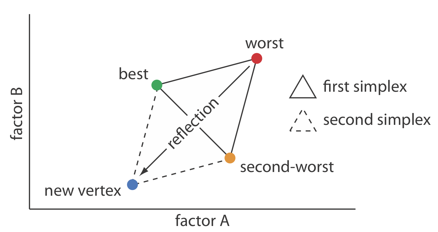
\(\newcommand{\avec}{\mathbf a}\) \(\newcommand{\bvec}{\mathbf b}\) \(\newcommand{\cvec}{\mathbf c}\) \(\newcommand{\dvec}{\mathbf d}\) \(\newcommand{\dtil}{\widetilde{\mathbf d}}\) \(\newcommand{\evec}{\mathbf e}\) \(\newcommand{\fvec}{\mathbf f}\) \(\newcommand{\nvec}{\mathbf n}\) \(\newcommand{\pvec}{\mathbf p}\) \(\newcommand{\qvec}{\mathbf q}\) \(\newcommand{\svec}{\mathbf s}\) \(\newcommand{\tvec}{\mathbf t}\) \(\newcommand{\uvec}{\mathbf u}\) \(\newcommand{\vvec}{\mathbf v}\) \(\newcommand{\wvec}{\mathbf w}\) \(\newcommand{\xvec}{\mathbf x}\) \(\newcommand{\yvec}{\mathbf y}\) \(\newcommand{\zvec}{\mathbf z}\) \(\newcommand{\rvec}{\mathbf r}\) \(\newcommand{\mvec}{\mathbf m}\) \(\newcommand{\zerovec}{\mathbf 0}\) \(\newcommand{\onevec}{\mathbf 1}\) \(\newcommand{\real}{\mathbb R}\) \(\newcommand{\twovec}[2]{\left[\begin{array}{r}#1 \\ #2 \end{array}\right]}\) \(\newcommand{\ctwovec}[2]{\left[\begin{array}{c}#1 \\ #2 \end{array}\right]}\) \(\newcommand{\threevec}[3]{\left[\begin{array}{r}#1 \\ #2 \\ #3 \end{array}\right]}\) \(\newcommand{\cthreevec}[3]{\left[\begin{array}{c}#1 \\ #2 \\ #3 \end{array}\right]}\) \(\newcommand{\fourvec}[4]{\left[\begin{array}{r}#1 \\ #2 \\ #3 \\ #4 \end{array}\right]}\) \(\newcommand{\cfourvec}[4]{\left[\begin{array}{c}#1 \\ #2 \\ #3 \\ #4 \end{array}\right]}\) \(\newcommand{\fivevec}[5]{\left[\begin{array}{r}#1 \\ #2 \\ #3 \\ #4 \\ #5 \\ \end{array}\right]}\) \(\newcommand{\cfivevec}[5]{\left[\begin{array}{c}#1 \\ #2 \\ #3 \\ #4 \\ #5 \\ \end{array}\right]}\) \(\newcommand{\mattwo}[4]{\left[\begin{array}{rr}#1 \amp #2 \\ #3 \amp #4 \\ \end{array}\right]}\) \(\newcommand{\laspan}[1]{\text{Span}\{#1\}}\) \(\newcommand{\bcal}{\cal B}\) \(\newcommand{\ccal}{\cal C}\) \(\newcommand{\scal}{\cal S}\) \(\newcommand{\wcal}{\cal W}\) \(\newcommand{\ecal}{\cal E}\) \(\newcommand{\coords}[2]{\left\{#1\right\}_{#2}}\) \(\newcommand{\gray}[1]{\color{gray}{#1}}\) \(\newcommand{\lgray}[1]{\color{lightgray}{#1}}\) \(\newcommand{\rank}{\operatorname{rank}}\) \(\newcommand{\row}{\text{Row}}\) \(\newcommand{\col}{\text{Col}}\) \(\renewcommand{\row}{\text{Row}}\) \(\newcommand{\nul}{\text{Nul}}\) \(\newcommand{\var}{\text{Var}}\) \(\newcommand{\corr}{\text{corr}}\) \(\newcommand{\len}[1]{\left|#1\right|}\) \(\newcommand{\bbar}{\overline{\bvec}}\) \(\newcommand{\bhat}{\widehat{\bvec}}\) \(\newcommand{\bperp}{\bvec^\perp}\) \(\newcommand{\xhat}{\widehat{\xvec}}\) \(\newcommand{\vhat}{\widehat{\vvec}}\) \(\newcommand{\uhat}{\widehat{\uvec}}\) \(\newcommand{\what}{\widehat{\wvec}}\) \(\newcommand{\Sighat}{\widehat{\Sigma}}\) \(\newcommand{\lt}{<}\) \(\newcommand{\gt}{>}\) \(\newcommand{\amp}{&}\) \(\definecolor{fillinmathshade}{gray}{0.9}\)One strategy for improving the efficiency of a searching algorithm is to change more than one factor at a time. A convenient way to accomplish this when there are two factors is to begin with three sets of initial factor levels arranged as the vertices of a triangle (Figure \(\PageIndex{1}\). After measuring the response for each set of factor levels, we identify the combination that gives the worst response and replace it with a new set of factor levels using a set of rules. This process continues until we reach the global optimum or until no further optimization is possible. The set of factor levels is called a simplex. In general, for k factors a simplex is a \(k + 1\) dimensional geometric figure [see Spendley, W.; Hext, G. R.; Himsworth, F. R. Technometrics 1962, 4, 441–461, and Deming, S. N.; Parker, L. R. CRC Crit. Rev. Anal. Chem. 1978 7(3), 187–202]. Thus, for two factors the simplex is a triangle. For three factors the simplex is a tetrahedron.
To place the initial two-factor simplex on the response surface, we choose a starting point (a, b) for the first vertex and place the remaining two vertices at (a + sa, b) and (a + 0.5sa, b + 0.87sb) where sa and sb are step sizes for factor A and for factor B [see, for example, Long, D. E. Anal. Chim. Acta 1969, 46, 193–206]. The following set of rules moves the simplex across the response surface in search of the optimum response:
Rule 1. Rank the vertices from best (vb) to worst (vw).
Rule 2. Reject the worst vertex (vw) and replace it with a new vertex (vn) by reflecting the worst vertex through the midpoint of the remaining vertices. The new vertex’s factor levels are twice the average factor levels for the retained vertices minus the factor levels for the worst vertex. For a two-factor optimization, the equations are shown here where vs is the third vertex.
\[a_{v_n} = 2 \left( \frac {a_{v_b} + a_{v_s}} {2} \right) - a_{v_w} \nonumber \]
\[b_{v_n} = 2 \left( \frac {b_{v_b} + b_{v_s}} {2} \right) - b_{v_w} \nonumber \]
Rule 3. If the new vertex has the worst response, then return to the previous vertex and reject the vertex with the second worst response, (vs) calculating the new vertex’s factor levels using rule 2. This rule ensures that the simplex does not return to the previous simplex.
Rule 4. Boundary conditions are a useful way to limit the range of possible factor levels. For example, it may be necessary to limit a factor’s concentration for solubility reasons, or to limit the temperature because a reagent is thermally unstable. If the new vertex exceeds a boundary condition, then assign it the worst response and follow rule 3.
Because the size of the simplex remains constant during the search, this algorithm is called a fixed-sized simplex optimization. The following example illustrates the application of these rules.
Find the optimum for the response surface described by the equation
\[R = 5.5 + 1.5 A + 0.6 B - 0.15 A^2 - 0.0254 B^2 - 0.0857 AB \nonumber \]
using the fixed-sized simplex searching algorithm. Use (0, 0) for the initial factor levels and set each factor’s step size to 1.00.
Solution
Letting a = 0, b =0, sa = 1.00, and sb = 1.00 gives the vertices for the initial simplex as
\[\text{vertex 1:} (a, b) = (0, 0) \nonumber\]
\[\text{vertex 2:} (a + s_a, b) = (1.00, 0) \nonumber\]
\[\text{vertex 3:} (a + 0.5s_a, b + 0.87s_b) = (0.50, 0.87) \nonumber\]
The responses for the three vertices are shown in the following table
| vertex | a | b | response |
|---|---|---|---|
| \(v_1\) | 0 | 0 | 5.50 |
| \(v_2\) | 1.00 | 0 | 6.85 |
| \(v_3\) | 0.50 | 0.87 | 6.68 |
with \(v_1\) giving the worst response and \(v_3\) the best response. Following Rule 1, we reject \(v_1\) and replace it with a new vertex; thus
\[a_{v_4} = 2 \left( \frac {1.00 + 0.50} {2} \right) - 0 = 1.50 \nonumber\]
\[b_{v_4} = 2 \left( \frac {0 + 0.87} {2} \right) - 0 = 0.87 \nonumber\]
The following table gives the vertices of the second simplex.
| vertex | a | b | response |
|---|---|---|---|
| \(v_2\) | 1.00 | 0 | 6.85 |
| \(v_3\) | 0.50 | 0.87 | 6.68 |
| \(v_4\) | 1.50 | 0.87 | 7.80 |
with \(v_3\) giving the worst response and \(v_4\) the best response. Following Rule 1, we reject \(v_3\) and replace it with a new vertex; thus
\[a_{v_5} = 2 \left( \frac {1.00 + 1.50} {2} \right) - 0.50 = 2.00 \nonumber\]
\[b_{v_5} = 2 \left( \frac {0 + 0.87} {2} \right) - 0.87 = 0 \nonumber\]
The following table gives the vertices of the third simplex.
| vertex | a | b | response |
|---|---|---|---|
| \(v_2\) | 1.00 | 0 | 6.85 |
| \(v_4\) | 1.50 | 0.87 | 7.80 |
| \(v_5\) | 2.00 | 0 | 7.90 |
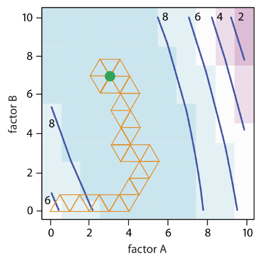
The calculation of the remaining vertices is left as an exercise. Figure \(\PageIndex{2}\) shows the progress of the complete optimization. After 29 steps the simplex begins to repeat itself, circling around the optimum response of (3, 7).
The size of the initial simplex ultimately limits the effectiveness and the efficiency of a fixed-size simplex searching algorithm. We can increase its efficiency by allowing the size of the simplex to expand or to contract in response to the rate at which we approach the optimum. For example, if we find that a new vertex is better than any of the vertices in the preceding simplex, then we expand the simplex further in this direction on the assumption that we are moving directly toward the optimum. Other conditions might cause us to contract the simplex—to make it smaller—to encourage the optimization to move in a different direction. We call this a variable-sized simplex optimization. Consult this chapter’s additional resources for further details of the variable-sized simplex optimization.