
9.5: Mathematical Models of Response Surfaces
- Page ID
- 290713

\( \newcommand{\vecs}[1]{\overset { \scriptstyle \rightharpoonup} {\mathbf{#1}} } \)
\( \newcommand{\vecd}[1]{\overset{-\!-\!\rightharpoonup}{\vphantom{a}\smash {#1}}} \)
\( \newcommand{\id}{\mathrm{id}}\) \( \newcommand{\Span}{\mathrm{span}}\)
( \newcommand{\kernel}{\mathrm{null}\,}\) \( \newcommand{\range}{\mathrm{range}\,}\)
\( \newcommand{\RealPart}{\mathrm{Re}}\) \( \newcommand{\ImaginaryPart}{\mathrm{Im}}\)
\( \newcommand{\Argument}{\mathrm{Arg}}\) \( \newcommand{\norm}[1]{\| #1 \|}\)
\( \newcommand{\inner}[2]{\langle #1, #2 \rangle}\)
\( \newcommand{\Span}{\mathrm{span}}\)
\( \newcommand{\id}{\mathrm{id}}\)
\( \newcommand{\Span}{\mathrm{span}}\)
\( \newcommand{\kernel}{\mathrm{null}\,}\)
\( \newcommand{\range}{\mathrm{range}\,}\)
\( \newcommand{\RealPart}{\mathrm{Re}}\)
\( \newcommand{\ImaginaryPart}{\mathrm{Im}}\)
\( \newcommand{\Argument}{\mathrm{Arg}}\)
\( \newcommand{\norm}[1]{\| #1 \|}\)
\( \newcommand{\inner}[2]{\langle #1, #2 \rangle}\)
\( \newcommand{\Span}{\mathrm{span}}\) \( \newcommand{\AA}{\unicode[.8,0]{x212B}}\)
\( \newcommand{\vectorA}[1]{\vec{#1}} % arrow\)
\( \newcommand{\vectorAt}[1]{\vec{\text{#1}}} % arrow\)
\( \newcommand{\vectorB}[1]{\overset { \scriptstyle \rightharpoonup} {\mathbf{#1}} } \)
\( \newcommand{\vectorC}[1]{\textbf{#1}} \)
\( \newcommand{\vectorD}[1]{\overrightarrow{#1}} \)
\( \newcommand{\vectorDt}[1]{\overrightarrow{\text{#1}}} \)
\( \newcommand{\vectE}[1]{\overset{-\!-\!\rightharpoonup}{\vphantom{a}\smash{\mathbf {#1}}}} \)
\( \newcommand{\vecs}[1]{\overset { \scriptstyle \rightharpoonup} {\mathbf{#1}} } \)
\( \newcommand{\vecd}[1]{\overset{-\!-\!\rightharpoonup}{\vphantom{a}\smash {#1}}} \)
\(\newcommand{\avec}{\mathbf a}\) \(\newcommand{\bvec}{\mathbf b}\) \(\newcommand{\cvec}{\mathbf c}\) \(\newcommand{\dvec}{\mathbf d}\) \(\newcommand{\dtil}{\widetilde{\mathbf d}}\) \(\newcommand{\evec}{\mathbf e}\) \(\newcommand{\fvec}{\mathbf f}\) \(\newcommand{\nvec}{\mathbf n}\) \(\newcommand{\pvec}{\mathbf p}\) \(\newcommand{\qvec}{\mathbf q}\) \(\newcommand{\svec}{\mathbf s}\) \(\newcommand{\tvec}{\mathbf t}\) \(\newcommand{\uvec}{\mathbf u}\) \(\newcommand{\vvec}{\mathbf v}\) \(\newcommand{\wvec}{\mathbf w}\) \(\newcommand{\xvec}{\mathbf x}\) \(\newcommand{\yvec}{\mathbf y}\) \(\newcommand{\zvec}{\mathbf z}\) \(\newcommand{\rvec}{\mathbf r}\) \(\newcommand{\mvec}{\mathbf m}\) \(\newcommand{\zerovec}{\mathbf 0}\) \(\newcommand{\onevec}{\mathbf 1}\) \(\newcommand{\real}{\mathbb R}\) \(\newcommand{\twovec}[2]{\left[\begin{array}{r}#1 \\ #2 \end{array}\right]}\) \(\newcommand{\ctwovec}[2]{\left[\begin{array}{c}#1 \\ #2 \end{array}\right]}\) \(\newcommand{\threevec}[3]{\left[\begin{array}{r}#1 \\ #2 \\ #3 \end{array}\right]}\) \(\newcommand{\cthreevec}[3]{\left[\begin{array}{c}#1 \\ #2 \\ #3 \end{array}\right]}\) \(\newcommand{\fourvec}[4]{\left[\begin{array}{r}#1 \\ #2 \\ #3 \\ #4 \end{array}\right]}\) \(\newcommand{\cfourvec}[4]{\left[\begin{array}{c}#1 \\ #2 \\ #3 \\ #4 \end{array}\right]}\) \(\newcommand{\fivevec}[5]{\left[\begin{array}{r}#1 \\ #2 \\ #3 \\ #4 \\ #5 \\ \end{array}\right]}\) \(\newcommand{\cfivevec}[5]{\left[\begin{array}{c}#1 \\ #2 \\ #3 \\ #4 \\ #5 \\ \end{array}\right]}\) \(\newcommand{\mattwo}[4]{\left[\begin{array}{rr}#1 \amp #2 \\ #3 \amp #4 \\ \end{array}\right]}\) \(\newcommand{\laspan}[1]{\text{Span}\{#1\}}\) \(\newcommand{\bcal}{\cal B}\) \(\newcommand{\ccal}{\cal C}\) \(\newcommand{\scal}{\cal S}\) \(\newcommand{\wcal}{\cal W}\) \(\newcommand{\ecal}{\cal E}\) \(\newcommand{\coords}[2]{\left\{#1\right\}_{#2}}\) \(\newcommand{\gray}[1]{\color{gray}{#1}}\) \(\newcommand{\lgray}[1]{\color{lightgray}{#1}}\) \(\newcommand{\rank}{\operatorname{rank}}\) \(\newcommand{\row}{\text{Row}}\) \(\newcommand{\col}{\text{Col}}\) \(\renewcommand{\row}{\text{Row}}\) \(\newcommand{\nul}{\text{Nul}}\) \(\newcommand{\var}{\text{Var}}\) \(\newcommand{\corr}{\text{corr}}\) \(\newcommand{\len}[1]{\left|#1\right|}\) \(\newcommand{\bbar}{\overline{\bvec}}\) \(\newcommand{\bhat}{\widehat{\bvec}}\) \(\newcommand{\bperp}{\bvec^\perp}\) \(\newcommand{\xhat}{\widehat{\xvec}}\) \(\newcommand{\vhat}{\widehat{\vvec}}\) \(\newcommand{\uhat}{\widehat{\uvec}}\) \(\newcommand{\what}{\widehat{\wvec}}\) \(\newcommand{\Sighat}{\widehat{\Sigma}}\) \(\newcommand{\lt}{<}\) \(\newcommand{\gt}{>}\) \(\newcommand{\amp}{&}\) \(\definecolor{fillinmathshade}{gray}{0.9}\)A response surface is described mathematically by an equation that relates the response to its factors. If we measure the response for several combinations of factor levels, then we can use a regression analysis to build a model of the response surface. There are two broad categories of models that we can use for a regression analysis: theoretical models and empirical models.
Theoretical Models of the Response Surface
A theoretical model is derived from the known chemical and physical relationships between the response and its factors. In spectrophotometry, for example, Beer’s law is a theoretical model that relates an analyte’s absorbance, A, to its concentration, CA
\[A = \epsilon b C_A \nonumber\]
where \(\epsilon\) is the molar absorptivity and b is the pathlength of the electromagnetic radiation passing through the sample. A Beer’s law calibration curve, therefore, is a theoretical model of a response surface. In Chapter 8 we learned how to use linear regression to build a mathematical model based on a theoretical relationship.
Empirical Models of the Response Surface
In many cases the underlying theoretical relationship between the response and its factors is unknown. We still can develop a model of the response surface if we make some reasonable assumptions about the underlying relationship between the factors and the response. For example, if we believe that the factors A and B are independent and that each has only a first-order effect on the response, then the following equation is a suitable model.
\[R = \beta_0 + \beta_a A + \beta_b B \nonumber\]
where R is the response, A and B are the factor levels, and \(\beta_0\), \(\beta_a\), and \(\beta_b\) are adjustable parameters whose values are determined by a linear regression analysis. Other examples of equations include those for dependent factors
\[R = \beta_0 + \beta_a A + \beta_b B + \beta_{ab} AB \nonumber\]
and those with higher-order terms.
\[R = \beta_0 + \beta_a A + \beta_b B + \beta_{aa} A^2 + \beta_{bb} B^2 \nonumber\]
Each of these equations provides an empirical model of the response surface because it has no rigorous basis in a theoretical understanding of the relationship between the response and its factors. Although an empirical model may provide an excellent description of the response surface over a limited range of factor levels, it has no basis in theory and we cannot reliably extend it to unexplored parts of the response surface.
Factorial Designs
To build an empirical model we measure the response for at least two levels for each factor. For convenience we label these levels as high, Hf, and low, Lf, where f is the factor; thus HA is the high level for factor A and LB is the low level for factor B. If our empirical model contains more than one factor, then each factor’s high level is paired with both the high level and the low level for all other factors. In the same way, the low level for each factor is paired with the high level and the low level for all other factors. As shown in Figure \(\PageIndex{1}\), this requires 2k experiments where k is the number of factors. This experimental design is known as a 2k factorial design.

Another system of notation is to use a plus sign (+) to indicate a factor’s high level and a minus sign (–) to indicate its low level.
Determining the Empirical Model
A 22 factorial design requires four experiments and allows for an empirical model with four variables.
With four experiments, we can use a 22 factorial design to create an empirical model that includes four variables: an intercept, first-order effects in A and B, and an interaction term between A and B
\[R = \beta_0 + \beta_a A + \beta_b B + \beta_{ab} AB \nonumber \]
The following example walks us through the calculations needed to find this model.
Suppose we wish to optimize the yield of a synthesis and we expect that the amount of catalyst (factor A with units of mM) and the temperature (factor B with units of °C) are likely important factors. The response, \(R\), is the reaction's yield in mg. We run four experiments and obtain the following responses:
| run | A | B | R |
|---|---|---|---|
| 1 | 15 | 20 | 145 |
| 2 | 25 | 20 | 158 |
| 3 | 15 | 30 | 135 |
| 4 | 25 | 30 | 150 |
Determine an equation for a response surface that provides a suitable model for predicting the effect of the catalyst and temperture on the reaction's yield.
Solution
Examining the data we see from runs 1 & 2 and from runs 3 & 4, that increasing factor A while holding factor B constant results in an increase in the response; thus, we expect that higher concentrations of the catalyst have a favorable affect on the reaction's yield. We also see from runs 1 & 3 and from runs 2 & 4, that increasing factor B while holding factor A constant results in a decrease in the response; thus, we expect that an increase in temperature has an unfavorable affect on the reaction's yield. Finally, we also see from runs 1 & 2 and from runs 3 & 4, that \(\Delta R\) is more positive when factor B is at its higher level; thus, we expect that there is a positive interaction between factors A and B. With four experiments, we are limited to a model that considers an intercept, first-order effects in A and B, and an interaction term between A and B
\[R = \beta_0 + \beta_a A + \beta_b B + \beta_{ab} AB \nonumber \]
We can work out values for this model's coefficients by solving the following set of simultaneous equations:
\[\beta_0 + 15 \beta_a + 20 \beta_b + (15)(20) \beta_{ab} = \beta_0 + 15 \beta_a + 20 \beta_b + 300 \beta_{ab} = 145 \nonumber \]
\[\beta_0 + 25 \beta_a + 20 \beta_b + (25)(20) \beta_{ab} = \beta_0 + 25 \beta_a + 20 \beta_b + 500 \beta_{ab} = 158 \nonumber \]
\[\beta_0 + 15 \beta_a + 30 \beta_b + (15)(30) \beta_{ab} = \beta_0 + 15 \beta_a + 30 \beta_b + 450 \beta_{ab} = 135 \nonumber \]
\[\beta_0 + 25 \beta_a + 30 \beta_b + (25)(30) \beta_{ab} = \beta_0 + 25 \beta_a + 30 \beta_b + 750 \beta_{ab} = 150 \nonumber \]
To solve this set of equations, we subtract the first equation from the second equation and subtract the third equation from the fourth equation, leaving us with the following two equations
\[10 \beta_a + 200 \beta_{ab} = 13 \nonumber \]
\[10 \beta_a + 300 \beta_{ab} = 15 \nonumber \]
Next, subtracting the first of these equations from the second gives
\[100 \beta_{ab} = 2 \nonumber \]
or \(\beta_{ab} = 0.02\). Substituting back gives
\[10 \beta_{a} + 200 \times 0.02 = 13 \nonumber \]
or \(\beta_a = 0.9\). Subtracting the equation for the first experiment from the equation for the third experiment gives
\[10 \beta_b + 150 \beta_{ab} = -10 \nonumber \]
Substituting in 0.02 for \(\beta_{ab}\) and solving gives \(\beta_b = -1.3\). Finally, substituting in our values for \(\beta_a\), \(\beta_b\), and \(\beta_{ab}\) into any of the first four equations gives \(\beta_0 = 151.5\). Our final model is
\[R = 151.5 + 0.9 A - 1.3 B + 0.02 AB \nonumber\]
When we consider how to interpret our empirical equation for the response surface, we need to consider several important limitations:
- The intercept in our model represents a condition far removed from our experiments: In this case, the intercept gives the reaction's yield in the absence of catalyst and at a temperature of 0°C, either of which we may not be useful conditions. In general, it is never a good idea to extrapolate a model far beyond the conditions used to define the model.
- The sign for a factor's first-order effects may be misleading if there is a significant interaction between it and other factors. Although our model shows that factor B (the temperature) has a negative first-order effect, the positive interaction between the two factors means there are conditions where an increase in B will increase the reaction's yield.
- It is difficult to judge the relative importance of two or more factors by examining their coefficients if their scales are not the same. This could present a problem, for example, if we reported the amount of catalyst (factor A) using molar concentrations as these values would be three-orders of magnitude smaller than the reported temperatures.
- When the number of variables is the same as the number of experiments, as is the case here, then there are no degrees of freedom and we have no simple way to test the model's suitability.
Determining the Empirical Model Using Coded Factor Levels
We can address two of the limitations described above by using coded factor levels in which we assign \(+1\) for a high level and \(-1\) for a low level. Defining the upper limit and the lower limit of the factors as \(+1\) and \(-1\) does two things for us: it places the intercept at the center of our experiments, which avoids the concern of extrapolating our model; and it places all factors on a common scale, and which makes it easier to compare the relative effects of the factors. Coding also makes it easier to determine the empirical model's equation when we complete calculations by hand.
To explore the effect of temperature on a reaction, we assign 30oC to a coded factor level of \(-1\) and assign a coded level \(+1\) to a temperature of 50oC. What temperature corresponds to a coded level of \(-0.5\) and what is the coded level for a temperature of 60oC?
Solution
The difference between \(-1\) and \(+1\) is 2, and the difference between 30oC and 50oC is 20oC; thus, each unit in coded form is equivalent to 10oC in uncoded form. With this information, it is easy to create a simple scale between the coded and the uncoded values, as shown in Figure \(\PageIndex{2}\). A temperature of 35oC corresponds to a coded level of \(-0.5\) and a coded level of \(+2\) corresponds to a temperature of 60oC.

As we see in the following example, factor levels simplify the calculations for an empirical model.
Rework Example \(\PageIndex{1}\) using coded factor levels.
Solution
The table below shows the original factor levels (A and B), their corresponding coded factor levels (A* and B*) and A*B*, which is the empirical model's interaction term.
| run | A | B | A* | B* | A*B* | R |
|---|---|---|---|---|---|---|
| 1 | 15 | 20 | \(-1\) | \(-1\) | \(+1\) | 145 |
| 2 | 25 | 20 | \(+1\) | \(-1\) | \(-1\) | 158 |
| 3 | 15 | 30 | \(-1\) | \(+1\) | \(-1\) | 135 |
| 4 | 25 | 30 | \(+1\) | \(+1\) | \(+1\) | 150 |
The empirical equation has four unknowns—the four beta terms—and Table \(\PageIndex{1}\) describes the four experiments. We have just enough information to calculate values for \(\beta_0\), \(\beta_a\), \(\beta_b\), and \(\beta_{ab}\). When working with the coded factor levels, the values of these parameters are easy to calculate using the following equations, where n is the number of runs.
\[\beta_{0} \approx b_{0}=\frac{1}{n} \sum_{i=1}^{n} R_{i} \nonumber \]
\[\beta_{a} \approx b_{a}=\frac{1}{n} \sum_{i=1}^{n} A^*_{i} R_{i} \nonumber \]
\[\beta_{b} \approx b_{b}=\frac{1}{n} \sum_{i=1}^{n} B^*_{i} R_{i} \nonumber \]
\[\beta_{ab} \approx b_{ab}=\frac{1}{n} \sum_{i=1}^{n} A^*_{i} B^*_{i} R_{i} \nonumber \]
Solving for the estimated parameters using the data in Table \(\PageIndex{1}\)
\[b_{0}=\frac{145 + 158 + 135 + 150}{4} = 147 \nonumber\]
\[b_{a}=\frac{-145 + 158 - 135 + 150}{4} = 7 \nonumber\]
\[b_{b}=\frac{-145 - 11.5 + 135 + 150}{4} = 5.0 \nonumber\]
\[b_{ab}=\frac{145 - 158 - 135 + 150}{4} = 0.5 \nonumber\]
leaves us with the coded empirical model for the response surface.
\[R = 147 + 7 A^* - 4.5 B^* + 0.5 A^* B^* \nonumber \]
Do you see why the equations for calculating \(b_0\), \(b_a\), \(b_b\), and \(b_{ab}\) work? Take the equation for \(b_a\) as an example
\[\beta_{a} \approx b_{a}=\frac{1}{n} \sum_{i=1}^{n} A^*_{i} R_{i} \nonumber \]
where
\[b_{a}=\frac{-145 + 158 - 135 + 150}{4} = 7 \nonumber\]
The first and the third terms in this equation give the response when \(A^*\) is at its low level, and the second and fourth terms in this equation give the response when \(A^*\) is at its high level. In the two terms where \(A^*\) is at its low level, \(B^*\) is at both its low level (first term) and its high level (third term), and in the two terms where \(A^*\) is at its high level, \(B^*\) is at both its low level (second term) and its high level (fourth term). As a result, the contribution of \(B^*\) is removed from the calculation. The same holds true for the effect of \(A^* B^*\), although this is left for you to confirm.
We can transform the coded model into a non-coded model by noting that \(A = 20 + 5A^*\) and that \(B = 25 + 5B^*\), solving for \(A^*\) and \(B^*\), to obtain \(A^* = 0.2 A - 4\) and \(B^* = 0.2 B - 5\), and substituting into the coded model and simplifying.
\[R = 147 + 7 (0.2A - 4) - 4.5 (0.2B - 5) + 0.5(0.2A - 4)(0.2A - 5) \nonumber\]
\[R = 147 + 1.4A - 28 - 0.9B + 22.5 + 0.02AB - 0.5A - 0.4B + 10 \nonumber\]
\[R = 151.5 + 0.9A - 1.3B + 0.02AB \nonumber \]
Note that this is the same equation that we derived in Example \(\PageIndex{1}\) using uncoded values for the factors.
Although we can convert this coded model into its uncoded form, there is no need to do so. If we want to know the response for a new set of factor levels, we just convert them into coded form and calculate the response. For example, if A is 23 and B is 22, then \(A^* = 02 \times 23 - 4 = 0.6\) and \(B^* = 0.2 \times 22 - 5 = -0.6\) and
\[R = 147 + 7 \times 0.6 - 4.5 \times (-0.6) + 0.5 \times 0.6 \times (-0.6) = 153.72 \approx 154 \text{ mg} \nonumber \]
We can extend this approach to any number of factors. For a system with three factors—A, B, and C—we can use a 23 factorial design to determine the parameters in the following empirical model
\[R = \beta_0 + \beta_a A + \beta_b B + \beta_c C + \beta_{ab} AB + \beta_{ac} AC + \beta_{bc} BC + \beta_{abc} ABC \nonumber \]
where A, B, and C are the factor levels. The terms \(\beta_0\), \(\beta_a\), \(\beta_b\), and \(\beta_{ab}\) are estimated using the following eight equations.
\[\beta_{0} \approx b_{0}=\frac{1}{n} \sum_{i=1}^{n} R_{i} \nonumber \]
\[\beta_{a} \approx b_{a}=\frac{1}{n} \sum_{i=1}^{n} A^*_{i} R_{i} \nonumber \]
\[\beta_{b} \approx b_{b}=\frac{1}{n} \sum_{i=1}^{n} B^*_{i} R_{i} \nonumber \]
\[\beta_{ab} \approx b_{ab}=\frac{1}{n} \sum_{i=1}^{n} A^*_{i} B^*_{i} R_{i} \nonumber \]
\[\beta_{c} \approx b_{c}=\frac{1}{n} \sum_{i=1}^{n} C^*_{i} R \nonumber \]
\[\beta_{ac} \approx b_{ac}=\frac{1}{n} \sum_{i=1}^{n} A^*_{i} C^*_{i} R \nonumber \]
\[\beta_{bc} \approx b_{bc}=\frac{1}{n} \sum_{i=1}^{n} B^*_{i} C^*_{i} R \nonumber \]
\[\beta_{abc} \approx b_{abc}=\frac{1}{n} \sum_{i=1}^{n} A^*_{i} B^*_{i} C^*_{i} R \nonumber \]
The following table lists the uncoded factor levels, the coded factor levels, and the responses for a 23 factorial design.
| run | A | B | C | A* | B* | C* | A*B* | A*C* | B*C* | A*B*C* | R |
|---|---|---|---|---|---|---|---|---|---|---|---|
| 1 | 15 | 30 | 45 | \(+1\) | \(+1\) | \(+1\) | \(+1\) |
\(+1\) |
\(+1\) |
\(+1\) |
137.5 |
| 2 | 15 | 30 | 15 | \(+1\) | \(+1\) | \(-1\) | \(+1\) | \(-1\) | \(-1\) | \(-1\) | 54.75 |
| 3 | 15 | 10 | 45 | \(+1\) | \(-1\) | \(+1\) | \(-1\) | \(+1\) | \(-1\) | \(-1\) | 73.75 |
| 4 | 15 | 10 | 15 | \(+1\) | \(-1\) | \(-1\) | \(-1\) | \(-1\) | \(+1\) | \(+1\) | 30.25 |
| 5 | 5 | 30 | 45 | \(-1\) | \(+1\) | \(+1\) | \(-1\) | \(-1\) | \(+1\) | \(-1\) | 61.75 |
| 6 | 5 | 30 | 15 | \(-1\) | \(+1\) | \(-1\) | \(-1\) | \(+1\) | \(-1\) | \(+1\) | 30.25 |
| 7 | 5 | 10 | 45 | \(-1\) | \(-1\) | \(+1\) | \(+1\) | \(-1\) | \(-1\) | \(+1\) | 41.25 |
| 8 | 5 | 10 | 15 | \(-1\) | \(-1\) | \(-1\) | \(+1\) | \(+1\) | \(+1\) | \(-1\) | 18.75 |
Determine the coded empirical model for the response surface based on the following equation.
\[R = \beta_0 + \beta_a A + \beta_b B + \beta_c C + \beta_{ab} AB + \beta_{ac} AC + \beta_{bc} BC + \beta_{abc} ABC \nonumber \]
What is the expected response when A is 10, B is 15, and C is 50?
Solution
The equation for the empirical model has eight unknowns—the eight beta terms—and the table above describes eight experiments. We have just enough information to calculate values for \(\beta_0\), \(\beta_a\), \(\beta_b\), \(\beta_{ab}\), \(\beta_{ac}\), \(\beta_{bc}\), and \(\beta_{abc}\); these values are
\[b_{0}=\frac{1}{8} \times(137.25+54.75+73.75+30.25+61.75+30.25+41.25+18.75 )=56.0 \nonumber\]
\[b_{a}=\frac{1}{8} \times(137.25+54.75+73.75+30.25-61.75-30.25-41.25-18.75 )=18.0 \nonumber\]
\[b_{b}=\frac{1}{8} \times(137.25+54.75-73.75-30.25+61.75+30.25-41.25-18.75 )=15.0 \nonumber\]
\[b_{c}=\frac{1}{8} \times(137.25-54.75+73.75-30.25+61.75-30.25+41.25-18.75 )=22.5 \nonumber\]
\[b_{ab}=\frac{1}{8} \times(137.25+54.75-73.75-30.25-61.75-30.25+41.25+18.75 )=7.0 \nonumber\]
\[b_{ac}=\frac{1}{8} \times(137.25-54.75+73.75-30.25-61.75+30.25-41.25+18.75 )=9.0 \nonumber\]
\[b_{bc}=\frac{1}{8} \times(137.25-54.75-73.75+30.25+61.75-30.25-41.25+18.75 )=6.0 \nonumber\]
\[b_{abc}=\frac{1}{8} \times(137.25-54.75-73.75+30.25-61.75+30.25+41.25-18.75 )=3.75 \nonumber\]
The coded empirical model, therefore, is
\[R = 56.0 + 18.0 A^* + 15.0 B^* + 22.5 C^* + 7.0 A^* B^* + 9.0 A^* C^* + 6.0 B^* C^* + 3.75 A^* B^* C^* \nonumber\]
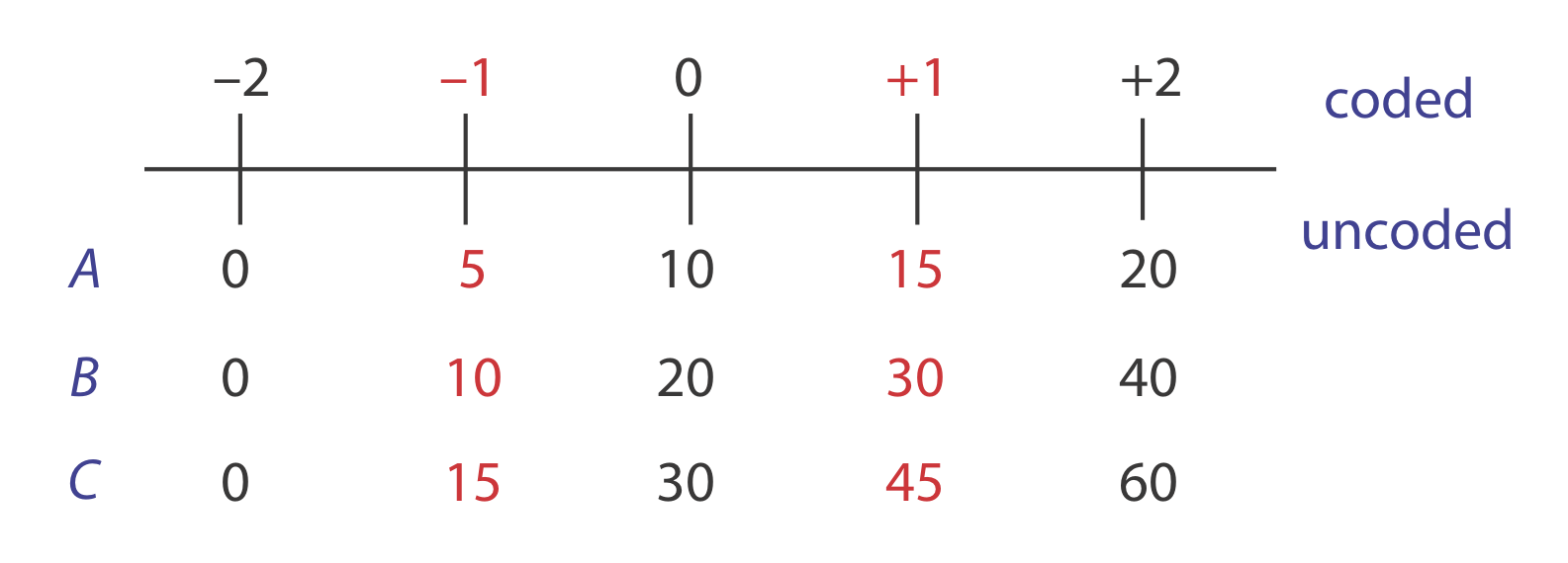
To find the response when A is 10, B is 15, and C is 50, we first convert these values into their coded form. Figure \(\PageIndex{3}\) helps us make the appropriate conversions; thus, A* is 0, B* is \(-0.5\), and C* is \(+1.33\). Substituting back into the empirical model gives a response of
\[R = 56.0 + 18.0 (0) + 15.0 (-0.5) + 22.5 (+1.33) + 7.0 (0) (-0.5) + 9.0 (0) (+1.33) + 6.0 (-0.5) (+1.33) + 3.75 (0) (-0.5) (+1.33) = 74.435 \approx 74.4 \nonumber\]
Evaluating an Empirical Model
A 2k factorial design can model only a factor’s first-order effect, including first-order interactions, on the response. A 22 factorial design, for example, includes each factor’s first-order effect (\(\beta_a\) and \(\beta_b\)) and a first-order interaction between the factors (\(\beta_{ab}\)). A 2k factorial design cannot model higher-order effects because there is insufficient information. Here is a simple example that illustrates the problem. Suppose we need to model a system in which the response is a function of a single factor, A. Figure \(\PageIndex{4a}\) shows the result of an experiment using a 21 factorial design. The only empirical model we can fit to the data is a straight line.
\[R = \beta_0 + \beta_a A \nonumber\]

If the actual response is a curve instead of a straight-line, then the empirical model is in error. To see evidence of curvature we must measure the response for at least three levels for each factor. We can fit the 31 factorial design in Figure \(\PageIndex{4b}\) to an empirical model that includes second-order factor effects.
\[R = \beta_0 + \beta_a A + \beta_{aa} A^2 \nonumber\]
In general, an n-level factorial design can model single-factor and interaction terms up to the (n – 1)th order.
We can judge the effectiveness of a first-order empirical model by measuring the response at the center of the factorial design. If there are no higher-order effects, then the average response of the trials in a 2k factorial design should equal the measured response at the center of the factorial design. To account for influence of random errors we make several determinations of the response at the center of the factorial design and establish a suitable confidence interval. If the difference between the two responses is significant, then a first-order empirical model probably is inappropriate.
One of the advantages of working with a coded empirical model is that b0 is the average response of the 2 \(\times\) k trials in a 2k factorial design.
One method for the quantitative analysis of vanadium is to acidify the solution by adding H2SO4 and oxidizing the vanadium with H2O2 to form a red-brown soluble compound with the general formula (VO)2(SO4)3. Palasota and Deming studied the effect of the relative amounts of H2SO4 and H2O2 on the solution’s absorbance, reporting the following results for a 22 factorial design [Palasota, J. A.; Deming, S. N. J. Chem. Educ. 1992, 62, 560–563].
| H2SO4 | H2O2 | absorbance |
|---|---|---|
| \(+1\) | \(+1\) | 0.330 |
| \(+1\) | \(-1\) | 0.359 |
| \(-1\) | \(+1\) | 0.293 |
| \(-1\) | \(-1\) | 0.420 |
Four replicate measurements at the center of the factorial design give absorbances of 0.334, 0.336, 0.346, and 0.323. Determine if a first-order empirical model is appropriate for this system. Use a 90% confidence interval when accounting for the effect of random error.
Solution
We begin by determining the confidence interval for the response at the center of the factorial design. The mean response is 0.335 with a standard deviation of 0.0094, which gives a 90% confidence interval of
\[\mu=\overline{X} \pm \frac{t s}{\sqrt{n}}=0.335 \pm \frac{(2.35)(0.0094)}{\sqrt{4}}=0.335 \pm 0.011 \nonumber\]
The average response, \(\overline{R}\), from the factorial design is
\[\overline{R}=\frac{0.330+0.359+0.293+0.420}{4}=0.350 \nonumber\]
Because \(\overline{R}\) exceeds the confidence interval’s upper limit of 0.346, we can reasonably assume that a 22 factorial design and a first-order empirical model are inappropriate for this system at the 95% confidence level.
Central Composite Designs
One limitation to a 3k factorial design, which would allow us to use an empirical model with second-order effects, is the number of trials we need to run. As shown in Figure \(\PageIndex{5}\), a 32 factorial design requires 9 trials. This number increases to 27 for three factors and to 81 for 4 factors.

A more efficient experimental design for a system that contains more than two factors is a central composite design, two examples of which are shown in Figure \(\PageIndex{6}\). The central composite design consists of a 2k factorial design, which provides data to estimate each factor’s first-order effect and interactions between the factors, and a star design that has \(2^k + 1\) points, which provides data to estimate second-order effects. Although a central composite design for two factors requires the same number of trials, nine, as a 32 factorial design, it requires only 15 trials and 25 trials when using three factors or four factors. See this chapter’s additional resources for details about the central composite designs.
