Home
Bookshelves
Analytical Chemistry
Chemometrics Using R (Harvey)
9: Optimizing Data
9.6: Using R to Model a Response Surface (Multiple Regression)

9.6: Using R to Model a Response Surface (Multiple Regression)

Last updated
Save as PDF

Page ID: 290715

$ \newcommand{\vecs}[1]{\overset { \scriptstyle \rightharpoonup} {\mathbf{#1}} } $

$ \newcommand{\vecd}[1]{\overset{-\!-\!\rightharpoonup}{\vphantom{a}\smash {#1}}} $

$ \newcommand{\id}{\mathrm{id}}$ $ \newcommand{\Span}{\mathrm{span}}$

( \newcommand{\kernel}{\mathrm{null}\,}\) $ \newcommand{\range}{\mathrm{range}\,}$

$ \newcommand{\RealPart}{\mathrm{Re}}$ $ \newcommand{\ImaginaryPart}{\mathrm{Im}}$

$ \newcommand{\Argument}{\mathrm{Arg}}$ $ \newcommand{\norm}[1]{\| #1 \|}$

$ \newcommand{\inner}[2]{\langle #1, #2 \rangle}$

$ \newcommand{\Span}{\mathrm{span}}$

$ \newcommand{\id}{\mathrm{id}}$

$ \newcommand{\Span}{\mathrm{span}}$

$ \newcommand{\kernel}{\mathrm{null}\,}$

$ \newcommand{\range}{\mathrm{range}\,}$

$ \newcommand{\RealPart}{\mathrm{Re}}$

$ \newcommand{\ImaginaryPart}{\mathrm{Im}}$

$ \newcommand{\Argument}{\mathrm{Arg}}$

$ \newcommand{\norm}[1]{\| #1 \|}$

$ \newcommand{\inner}[2]{\langle #1, #2 \rangle}$

$ \newcommand{\Span}{\mathrm{span}}$ $ \newcommand{\AA}{\unicode[.8,0]{x212B}}$

$ \newcommand{\vectorA}[1]{\vec{#1}} % arrow$

$ \newcommand{\vectorAt}[1]{\vec{\text{#1}}} % arrow$

$ \newcommand{\vectorB}[1]{\overset { \scriptstyle \rightharpoonup} {\mathbf{#1}} } $

$ \newcommand{\vectorC}[1]{\textbf{#1}} $

$ \newcommand{\vectorD}[1]{\overrightarrow{#1}} $

$ \newcommand{\vectorDt}[1]{\overrightarrow{\text{#1}}} $

$ \newcommand{\vectE}[1]{\overset{-\!-\!\rightharpoonup}{\vphantom{a}\smash{\mathbf {#1}}}} $

$ \newcommand{\vecs}[1]{\overset { \scriptstyle \rightharpoonup} {\mathbf{#1}} } $

$ \newcommand{\vecd}[1]{\overset{-\!-\!\rightharpoonup}{\vphantom{a}\smash {#1}}} $

$\newcommand{\avec}{\mathbf a}$ $\newcommand{\bvec}{\mathbf b}$ $\newcommand{\cvec}{\mathbf c}$ $\newcommand{\dvec}{\mathbf d}$ $\newcommand{\dtil}{\widetilde{\mathbf d}}$ $\newcommand{\evec}{\mathbf e}$ $\newcommand{\fvec}{\mathbf f}$ $\newcommand{\nvec}{\mathbf n}$ $\newcommand{\pvec}{\mathbf p}$ $\newcommand{\qvec}{\mathbf q}$ $\newcommand{\svec}{\mathbf s}$ $\newcommand{\tvec}{\mathbf t}$ $\newcommand{\uvec}{\mathbf u}$ $\newcommand{\vvec}{\mathbf v}$ $\newcommand{\wvec}{\mathbf w}$ $\newcommand{\xvec}{\mathbf x}$ $\newcommand{\yvec}{\mathbf y}$ $\newcommand{\zvec}{\mathbf z}$ $\newcommand{\rvec}{\mathbf r}$ $\newcommand{\mvec}{\mathbf m}$ $\newcommand{\zerovec}{\mathbf 0}$ $\newcommand{\onevec}{\mathbf 1}$ $\newcommand{\real}{\mathbb R}$ $\newcommand{\twovec}[2]{\left[\begin{array}{r}#1 \\ #2 \end{array}\right]}$ $\newcommand{\ctwovec}[2]{\left[\begin{array}{c}#1 \\ #2 \end{array}\right]}$ $\newcommand{\threevec}[3]{\left[\begin{array}{r}#1 \\ #2 \\ #3 \end{array}\right]}$ $\newcommand{\cthreevec}[3]{\left[\begin{array}{c}#1 \\ #2 \\ #3 \end{array}\right]}$ $\newcommand{\fourvec}[4]{\left[\begin{array}{r}#1 \\ #2 \\ #3 \\ #4 \end{array}\right]}$ $\newcommand{\cfourvec}[4]{\left[\begin{array}{c}#1 \\ #2 \\ #3 \\ #4 \end{array}\right]}$ $\newcommand{\fivevec}[5]{\left[\begin{array}{r}#1 \\ #2 \\ #3 \\ #4 \\ #5 \\ \end{array}\right]}$ $\newcommand{\cfivevec}[5]{\left[\begin{array}{c}#1 \\ #2 \\ #3 \\ #4 \\ #5 \\ \end{array}\right]}$ $\newcommand{\mattwo}[4]{\left[\begin{array}{rr}#1 \amp #2 \\ #3 \amp #4 \\ \end{array}\right]}$ $\newcommand{\laspan}[1]{\text{Span}\{#1\}}$ $\newcommand{\bcal}{\cal B}$ $\newcommand{\ccal}{\cal C}$ $\newcommand{\scal}{\cal S}$ $\newcommand{\wcal}{\cal W}$ $\newcommand{\ecal}{\cal E}$ $\newcommand{\coords}[2]{\left\{#1\right\}_{#2}}$ $\newcommand{\gray}[1]{\color{gray}{#1}}$ $\newcommand{\lgray}[1]{\color{lightgray}{#1}}$ $\newcommand{\rank}{\operatorname{rank}}$ $\newcommand{\row}{\text{Row}}$ $\newcommand{\col}{\text{Col}}$ $\renewcommand{\row}{\text{Row}}$ $\newcommand{\nul}{\text{Nul}}$ $\newcommand{\var}{\text{Var}}$ $\newcommand{\corr}{\text{corr}}$ $\newcommand{\len}[1]{\left|#1\right|}$ $\newcommand{\bbar}{\overline{\bvec}}$ $\newcommand{\bhat}{\widehat{\bvec}}$ $\newcommand{\bperp}{\bvec^\perp}$ $\newcommand{\xhat}{\widehat{\xvec}}$ $\newcommand{\vhat}{\widehat{\vvec}}$ $\newcommand{\uhat}{\widehat{\uvec}}$ $\newcommand{\what}{\widehat{\wvec}}$ $\newcommand{\Sighat}{\widehat{\Sigma}}$ $\newcommand{\lt}{<}$ $\newcommand{\gt}{>}$ $\newcommand{\amp}{&}$ $\definecolor{fillinmathshade}{gray}{0.9}$

The calculations for determining an empirical model of a response surface using a 2^k factorial design, as outlined in Section 9.5, are relatively easy to complete for a small number of factors and for experimental designs without replication where the number of experiments is equal to the number of parameters in the model. If we wish to work with more factors, if we wish to explore other experimental designs, and if we wish to build replication into the experimental design so that we can better evaluate our empirical model, then we need to do so by building a regression model, as we did earlier in Chapter 8.

Creating Empirical Models Using R

To illustrate how we can use R to create an empirical model, let's use data from an experiment exploring how to optimize a Grignard reaction leading to the synthesis of benzyl-1-cyclopentan-1-ol [Bouzidi, N.; Gozzi, C. J. Chem. Educ. 2008, 85, 1544–1547]. In this study, students begin by studying the effect of six possible factors on the reaction's yield: the volume of diethyl ether used to prepare a solution of benzyl chloride, $x_1$, the time over which benzyl chloride is added to the reaction mixture, $x_2$, the stirring time used to prepare the benzyl magnesium chloride, $x_3$, the relative excess of benzyl chloride to cyclopentanone, $x_4$, the relative excess of magnesium turnings to benzyl chloride, $x_5$, and the reaction time, $x_6$.

With six factors to consider, a full 2^k factorial design requires 32 experiments, which is labor intensive. Instead, the students begin with a screening study that uses eight experiments to model only the first-order effects of the six factors, as outlined in the following two tables.

Table $\PageIndex{1}$: Factor Levels for Screening Study
factor	low level	high levcel
$x_1$: volume of diethyl ether in mL	18	50
$x_2$: addition time in min	60	90
$x_3$: stirring time in min	20	40
$x_4$: relative excess of benzyl chloride as %	20	30
$x_5$: relative excess of magnesium as %	12.5	25
$x_6$: reaction time in min	30	60

Table $\PageIndex{2}$: Experimental Design Showing Coded Factor Levels and Responses
run	$x_1$	$x_2$	$x_3$	$x_4$	$x_5$	$x_6$	percent yield
1	$+1$	$+1$	$+1$	$-1$	$+1$	$-1$	72
2	$-1$	$+1$	$+1$	$+1$	$-1$	$+1$	33
3	$-1$	$-1$	$+1$	$+1$	$+1$	$-1$	29
4	$+1$	$-1$	$-1$	$+1$	$+1$	$+1$	74
5	$-1$	$+1$	$-1$	$-1$	$+1$	$+1$	31
6	$+1$	$+1$	$+1$	$-1$	$-1$	$+1$	52
7	$+1$	$-1$	$-1$	$+1$	$-1$	$-1$	47
8	$-1$	$-1$	$-1$	$-1$	$-1$	$-1$	27

To carry out the calculations in R we first create vectors for the coded factor levels and the responses.

x1 = c(1,-1,-1,1,-1,1,1,-1) x2 = c(1,1,-1,-1,1,-1,1,-1) x3 = c(1,1,1,-1,-1,1,-1,-1) x4 = c(-1,1,1,1,-1,-1,1,-1) x5 = c(1,-1,1,1,1,-1,-1,-1) x6 = c(-1,1,-1,1,1,1,-1,-1) yield = c(72,33,29,74,31,52,47,27)

Next, we use the lm() function to build a linear regression model that includes just the first-order effects of the factors (see Chapter 8.5 to review the syntax for this function), and the summary() function to review the resulting model.

screening = lm(yield ~ x1 + x2 + x3 + x4 + x5 + x6) summary(screening)

Call:

lm(formula = yield ~ x1 + x2 + x3 + x4 + x5 + x6)

Residuals:

1 2 3 4 5 6 7 8

5.875 5.875 -5.875 5.875 -5.875 -5.875 -5.875 5.875

Coefficients:

Estimate Std.Error t value Pr(>|t|)

(Intercept) 45.625 5.875 7.766 0.0815 .

x1 15.625 5.875 2.660 0.2290

x2 0.125 5.875 0.021 0.9865

x3 0.875 5.875 0.149 0.9059

x4 0.125 5.875 0.021 0.9865

x5 5.875 5.875 1.000 0.5000

x6 1.875 5.875 0.319 0.8033

---

Signif. codes: 0 ‘***’ 0.001 ‘**’ 0.01 ‘*’ 0.05 ‘.’ 0.1 ‘ ’ 1

Residual standard error: 16.62 on 1 degrees of freedom

Multiple R-squared: 0.8913, Adjusted R-squared: 0.239

F-statistic: 1.366 on 6 and 1 DF, p-value: 0.5749

Because we have one more experiment than there are variables in our empirical model, the summary provides some information on the significance of the model's parameters; however, with just one degree of freedom this information is not really reliable. In addition to the intercept, the three factors with the largest coefficients are the volume of diethyl ether, $x_1$, the relative excess of magnesium, $x_5$, and the reaction time, $x_6$.

Having identified three factors for further investigation, the students use a 2³ factorial design to explore interactions between these three factors using the experimental design in the following table (see Table $\PageIndex{1}$ for the actual factor levels.

Table $\PageIndex{3}$: Coded Factor Levels and Response for a $2^3$ Factorial Design
run	$x_1$	$x_5$	$x_6$	percent yield
1	$-1$	$-1$	$-1$	28.5
2	$+1$	$-1$	$-1$	55.5
3	$-1$	$+1$	$-1$	38
4	$+1$	$+1$	$-1$	68
5	$-1$	$-1$	$+1$	49
6	$+1$	$-1$	$+1$	66
7	$-1$	$+1$	$+1$	31.5
8	$+1$	$+1$	$+1$	72

As before, we create vectors for our factors and the response and then use the lm() and the summary() functions to complete and evaluate the resulting empirical model.

x1 = c(-1,1,-1,1,-1,1,-1,1) x5 = c(-1,-1,1,1,-1,-1,1,1) x6 = c(-1,-1,-1,-1,1,1,1,1) yield = c(28.5,55.5,38,68,49,66,31.5,72) fact23 = lm(yield ~ x1 * x5 * x6) summary(fact23)

Call:

lm(formula = yield ~ x1 * x5 * x6)

Residuals:

ALL 8 residuals are 0: no residual degrees of freedom!

Coefficients:

Estimate Std. Error t value Pr(>|t|)

(Intercept) 51.0625 NA NA NA

x1 14.3125 NA NA NA

x5 1.3125 NA NA NA

x6 3.5625 NA NA NA

x1:x5 3.3125 NA NA NA

x1:x6 0.0625 NA NA NA

x5:x6 -4.1875 NA NA NA

x1:x5:x6 2.5625 NA NA NA

Residual standard error: NaN on 0 degrees of freedom

Multiple R-squared: 1, Adjusted R-squared: NaN

F-statistic: NaN on 7 and 0 DF, p-value: NA

With eight experiments and eight variables in the empirical model, we do not have any ability to evaluate the model statistically. Of the three first-order effects, we see that the volume of diethyl ether, $x_1$, and reaction time, $x_6$, are more important than the relative excess of magnesium, $x_5$. We also see that the interaction between $x_1$ and $x_5$ is positive (high values for both favor an increased yield) and that the interaction between $x_5$ and $x_6$ is negative (yields improve when one factor is high and the other is low).

Finally, the students use a central composite model—which allows for adding second-order effects and curvature in the response surface—to study the effect of the volume of diethyl ether, $x_1$, and reaction time, $x_6$, on the percent yield. The relative excess of magnesium, $x_5$ was set at its high level for this study because this provides for greater percent yields (compare the results for runs 4 and 6 to the results for runs 3 and 5 in Table $\PageIndex{3}$). The following tables provides the experimental design.

Table $\PageIndex{4}$: Coded Factor Levels and Responses for a Central Composite Experimental Design
run	$x_1$	$x_6$	percent yield
1	$-1$	$-1$	39
2	$+1$	$-1$	66.5
3	$-1$	$+1$	22
4	$+1$	$+1$	72.5
5	$-1.414$	0	10.5
6	$+1.414$	0	72.5
7	0	$-1.414$	38
8	0	$+1.414$	70
9	0	0	59
10	0	0	57
11	0	0	54.5
12	0	0	63

As before, we create vectors for our factors and the response, and then use the lm() and the summary() functions to complete and evaluate the resulting empirical model.

x1 = c(-1,1,-1,1,-1.414,1.414,0,0,0,0,0,0) x6 = c(-1,-1,1,1,0,0,-1.414,1.414,0,0,0,0) yield = c(39,66.5,22,72.5,10.5,72.5,38,70,59,57,54.5,63) centcomp = lm(yield ~ x1 * x6 + I(x1^2) + I(x6^2)) summary(centcomp)

Call:

lm(formula = yield ~ x1 * x6 + I(x1^2) + I(x6^2))

Residuals:

Min 1Q Median 3Q Max

-11.0724 -4.0794 -0.3938 5.2056 9.3695

Coefficients:

Estimate Std. Error t value Pr(>|t|)

(Intercept) 58.375 4.360 13.389 1.07e-05 ***

x1 20.712 3.083 6.718 0.000529 ***

x6 4.282 3.083 1.389 0.214267

I(x1^2) -7.876 3.447 -2.285 0.062398 .

I(x6^2) -1.625 3.447 -0.471 0.654130

x1:x6 5.750 4.360 1.319 0.235317

---

Signif. codes: 0 ‘***’ 0.001 ‘**’ 0.01 ‘*’ 0.05 ‘.’ 0.1 ‘ ’ 1

Residual standard error: 8.72 on 6 degrees of freedom

Multiple R-squared: 0.9, Adjusted R-squared: 0.8167

F-statistic: 10.8 on 5 and 6 DF, p-value: 0.005835

With 12 experiments and just six variables, our model has sufficient degrees of freedom to suggest that it provides a reasonable picture of how the reaction time and the volume of diethyl ether affect the reaction's yield even if the residual errors in the responses range from a minimum of -11.7 to a maximum +9.37. The middle 50% of residual errors range between -4.1 to +5.2 with a median residual error of -0.4. We can compare the actual experimental yields to the yields predicted by the model by combining them into a data frame.

centcomp_results = data.frame(yield, centcomp$fitted.values, yield - centcomp$fitted.values) colnames(centcomp_results) = c("expt yield", "pred yield", "residual error") centcomp_results

expt yield pred yield residual error

1 39.0 29.63046 9.3695385

2 66.5 59.55372 6.9462836

3 22.0 26.69375 -4.6937546

4 72.5 79.61701 -7.1170095

5 10.5 13.34036 -2.8403635

6 72.5 71.91285 0.5871540

7 38.0 49.07236 -11.0723566

8 70.0 61.18085 8.8191471

9 59.0 58.37466 0.6253402

10 57.0 58.37466 -1.3746598

11 54.5 58.37466 -3.8746598

12 63.0 58.37466 4.6253402

Using R to Visualize the Response Surface

The plot3D package provides several functions that we can use to visualize a response surface defined by two factors. Here we consider three functions, one for drawing a two-dimensional contour plot of the response surface, one for drawing a three-dimensional surface plot of the response, and one for plotting a three-dimensional scatter plot of the responses. To begin, we use the library() function to make the package available to us (note: you may need to first install the plot3D package; see Chapter 1 for details on how to do this).

library(plot3D)

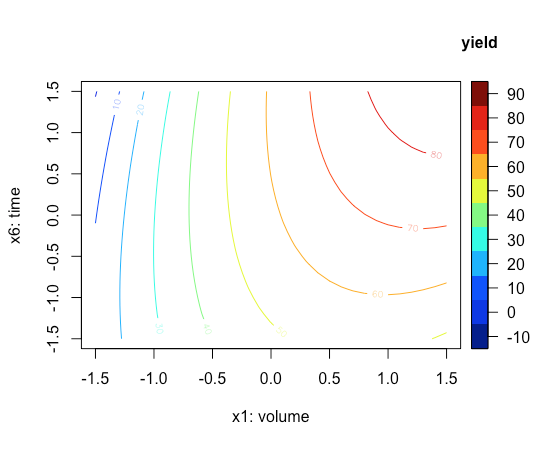
Let's begin by creating a two-dimensional contour plot of our response surface that places the volume of diethyl ether, $x_1$, on the x-axis and the reaction time, $x_6$ on the y-axis, and using calculated responses from the model to draw the contour lines. First, we create vectors with values for the x-axis and the y-axis

x1_axis = seq(-1.5, 1.5, 0.1) x6_axis = seq(-1.5 ,1.5, 0.1)

Next, we create a function that uses our empirical model to calculate the response for every combination of x1_axis and x6_axis

response = function(x,y){coef(centcomp)[1] + coef(centcomp)[2]*x + coef(centcomp)[3]*y + coef(centcomp)[4]*x^2 + coef(centcomp)[5]*y^2 + coef(centcomp)[6]*x*y}

where coef(centcomp)[i] is used to extract the i^th coefficient from our empirical model. Now we use R's outer() function to calculate the response for every combination of the variables x1_axis and x6_axis

z_axis = outer(X = x1_axis,Y = x6_axis, response)

Finally, we use the contour2D() function to create the contour plot in Figure $\PageIndex{1}$.

contour2D(x = x1_axis,y = x6_axis, z = z_axis, xlab = "x1: volume", ylab = "x6: time", clab = "yield")

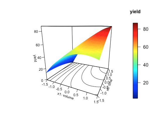
Figure $\PageIndex{1}$: Contour plot for the response surface predicting the percent yield in a Grignard reaction as a function of the volume of diethyl ether and the reaction time. The x-axis and the y-axis values are coded factor levels.

Next, let's create a three-dimensional surface plot of our response surface that places the volume of diethyl ether, $x_1$, on the x-axis, the reaction time, $x_6$ on the y-axis, and the calculated responses from the model on the z-axis. For this, we use the persp3D() function

persp3D(x = x1_axis, y = x6_axis, z = z_axis, ticktype = "detailed", phi = 15, theta = 25, xlab = "x1: volume", ylab = "x6: time", zlab = "yield", clab = "yield", contour = TRUE, cex.axis = 0.75, cex.lab = 0.75)

where phi and theta adjust the angle at which we view the response surface—you will have to play with these values to create a plot that is pleasing to look at—and ticktype controls how much information is displayed on the axes. The cex.axis and cex.lab commands adjust the size of the text displayed on the axes, and countour = TRUE places a contour plot on the figure's bottom side. Figure $\PageIndex{2}$ shows the result.

Figure $\PageIndex{2}$: Three-dimensional surface (perspective) plot for the response surface predicting the percent yield in a Grignard reaction as a function of the volume of diethyl ether and the reaction time. The x-axis and the y-axis values are coded factor levels.

Finally, let's use the type = "h" option to overlay a scatterplot of the data used to build the empirical model on top of the three-dimensional surface plot.

scatter3D(x = x1, y = x6, z = yield, add = TRUE, type = "h", pch = 19, col = "black", lwd = 2, colkey = FALSE)

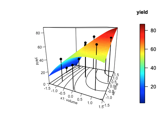
Figure $\PageIndex{3}$: Three-dimensional surface (perspective) plot for the response surface predicting the percent yield in a Grignard reaction as a function of the volume of diethyl ether and the reaction time showing the original data used to build the empirical model. The x-axis and the y-axis values are coded factor levels.

Figure $\PageIndex{3}$ shows the result using the data from Table $\PageIndex{4}$. Although the general shape of the response surface is consistent with the underlying data, there is sufficient experimental uncertainty in the results of the four replicate experiments used to create this empirical model, as shown by the standard deviation for runs 9—12, to explain why some of the predicted yields have large errors.

sd(yield[9:12])

[1] 3.591077

run	\(x_1\)	\(x_2\)	\(x_3\)	\(x_4\)	\(x_5\)	\(x_6\)	percent yield
1	\(+1\)	\(+1\)	\(+1\)	\(-1\)	\(+1\)	\(-1\)	72
2	\(-1\)	\(+1\)	\(+1\)	\(+1\)	\(-1\)	\(+1\)	33
3	\(-1\)	\(-1\)	\(+1\)	\(+1\)	\(+1\)	\(-1\)	29
4	\(+1\)	\(-1\)	\(-1\)	\(+1\)	\(+1\)	\(+1\)	74
5	\(-1\)	\(+1\)	\(-1\)	\(-1\)	\(+1\)	\(+1\)	31
6	\(+1\)	\(+1\)	\(+1\)	\(-1\)	\(-1\)	\(+1\)	52
7	\(+1\)	\(-1\)	\(-1\)	\(+1\)	\(-1\)	\(-1\)	47
8	\(-1\)	\(-1\)	\(-1\)	\(-1\)	\(-1\)	\(-1\)	27

run	\(x_1\)	\(x_5\)	\(x_6\)	percent yield
1	\(-1\)	\(-1\)	\(-1\)	28.5
2	\(+1\)	\(-1\)	\(-1\)	55.5
3	\(-1\)	\(+1\)	\(-1\)	38
4	\(+1\)	\(+1\)	\(-1\)	68
5	\(-1\)	\(-1\)	\(+1\)	49
6	\(+1\)	\(-1\)	\(+1\)	66
7	\(-1\)	\(+1\)	\(+1\)	31.5
8	\(+1\)	\(+1\)	\(+1\)	72

Search

Text Color

Text Size

Margin Size

Font Type

factor	low level	high levcel
\(x_1\): volume of diethyl ether in mL	18	50
\(x_2\): addition time in min	60	90
\(x_3\): stirring time in min	20	40
\(x_4\): relative excess of benzyl chloride as %	20	30
\(x_5\): relative excess of magnesium as %	12.5	25
\(x_6\): reaction time in min	30	60