9.3: One-Factor-at-a-Time Optimizations

A simple algorithm for optimizing the quantitative method for vanadium described earlier is to select initial concentrations for H₂O₂ and H₂SO₄ and measure the absorbance. Next, we optimize one reagent by increasing or decreasing its concentration—holding constant the second reagent’s concentration—until the absorbance decreases. We then vary the concentration of the second reagent—maintaining the first reagent’s optimum concentration—until we no longer see an increase in the absorbance. We can stop this process, which we call a one-factor-at-a-time optimization, after one cycle or repeat the steps until the absorbance reaches a maximum value or it exceeds an acceptable threshold value.

A one-factor-at-a-time optimization is consistent with a notion that to determine the influence of one factor we must hold constant all other factors. This is an effective, although not necessarily an efficient experimental design when the factors are independent [see Sharaf, M. A.; Illman, D. L.; Kowalski, B. R. Chemometrics, Wiley-Interscience: New York, 1986]. Two factors are independent when a change in the level of one factor does not influence the effect of a change in the other factor’s level. Table \(\PageIndex{1}\) provides an example of two independent factors.

Table \(\PageIndex{1}\). Example of Two Independent Factors

factor A	factor B	response
\(A_1\)	\(B_1\)	40
\(A_2\)	\(B_1\)	80
\(A_1\)	\(B_2\)	60
\(A_2\)	\(B_2\)	100

If we hold factor B at level B₁, changing factor A from level A₁ to level A₂ increases the response from 40 to 80, or a change in response, \(\Delta R\) of

\[R = 80 - 40 = 40 \nonumber\]

If we hold factor B at level B₂, we find that we have the same change in response when the level of factor A changes from A₁ to A₂.

\[R = 100 - 60 = 40 \nonumber\]

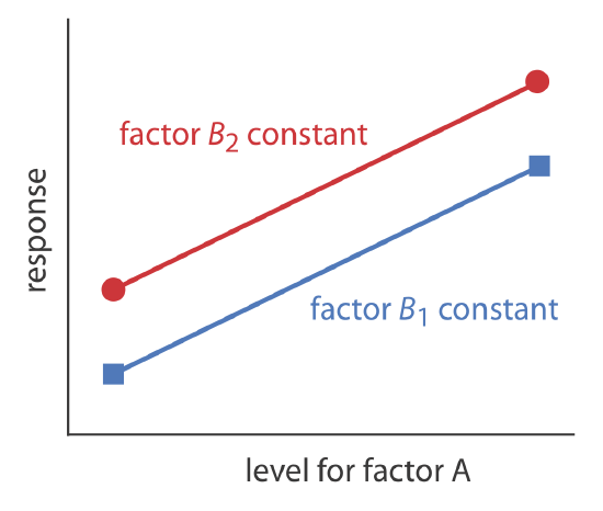
We can see this independence visually if we plot the response as a function of factor A’s level, as shown in Figure \(\PageIndex{1}\). The parallel lines show that the level of factor B does not influence factor A’s effect on the response.

Figure \(\PageIndex{1}\). Factor effect plot for two independent factors. Note that the two lines are parallel, indicating that the level for factor B does not influence how factor A’s level affects the response.

Mathematically, two factors are independent if they do not appear in the same term in the equation that describes the response surface. Figure \(\PageIndex{2}\), for example, shows the resulting pseudo-three-dimensional surface and a contour map for the equation

\[R = 2.0 + 0.12 A + 0.48 B - 0.03A^2 - 0.03 B^2 \nonumber \]

which describes a response surface with independent factors because no term in the equation includes both factor A and factor B.

Figure \(\PageIndex{2}\). The response surface for two independent factors based on the equation \(R = 2.0 + 0.12 A + 0.48 B - 0.03A^2 - 0.03 B^2\) and displayed as (a) a wireframe, and as (b) an overlaid contour plot and level plot. The orange lines in (b) show the progress of one-factor-at-a-time optimizations beginning from two starting points (•) and optimizing factor A first (solid line) or factor B first (dashed line). All four trials reach the optimum response of (2,8) in a single cycle.

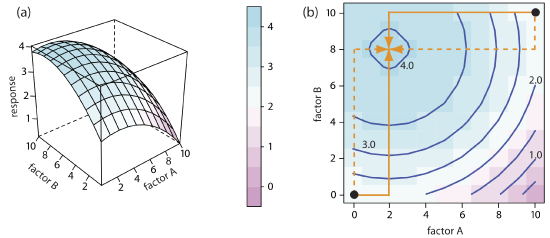
The easiest way to follow the progress of a searching algorithm is to map its path on a contour plot of the response surface. Positions on the response surface are identified as (a, b) where a and b are the levels for factor A and for factor B. The contour plot in Figure \(\PageIndex{2b}\), for example, shows four one-factor-at-a-time optimizations of the response surface in Figure \(\PageIndex{2a}\). The effectiveness and efficiency of this algorithm when optimizing independent factors is clear—each trial reaches the optimum response at (2, 8) in a single cycle.

Unfortunately, factors often are not independent. Consider, for example, the data in Table \(\PageIndex{2}\)

Table \(\PageIndex{2}\). Example of Two Dependent Factors

factor A	factor B	response
\(A_1\)	\(B_1\)	20
\(A_2\)	\(B_1\)	80
\(A_1\)	\(B_2\)	60
\(A_2\)	\(B_2\)	80

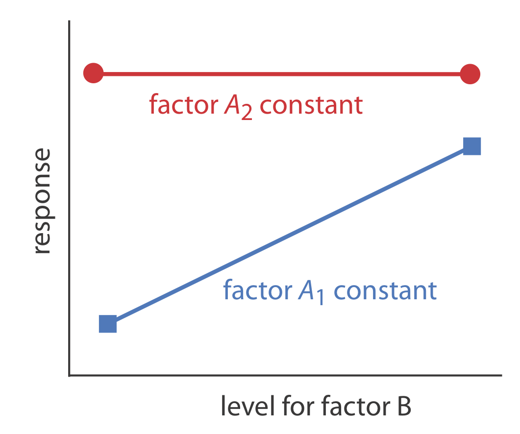
where a change in the level of factor B from level B₁ to level B₂ has a significant effect on the response when factor A is at level A₁

\[R = 60 - 20 = 40 \nonumber\]

but no effect when factor A is at level A₂.

\[R = 80 - 80 = 0 \nonumber\]Figure \(\PageIndex{3}\) shows this dependent relationship between the two factors.

Figure \(\PageIndex{3}\). Factor effect plot for two dependent factors. Note that the two lines are not parallel, indicating that the level for factor A influences how factor B’s level affects the response.

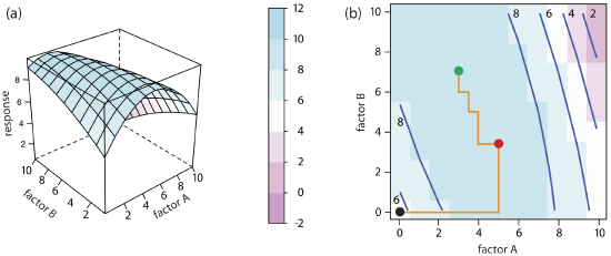
Factors that are dependent are said to interact and the equation for the response surface includes an interaction term that contains both factor A and factor B. The final term in this equation

\[R = 5.5 + 1.5 A + 0.6 B - 0.15 A^2 - 0.245 B^2 - 0.0857 AB \nonumber \]

for example, accounts for the interaction between factor A and factor B. Figure \(\PageIndex{4}\) shows the resulting pseudo-three-dimensional surface and a contour map for the response surface defined by this equation. The progress of a one-factor-at-a-time optimization for this response surface is shown in Figure \(\PageIndex{4b}\). Although the optimization for dependent factors is effective, it is less efficient than that for independent factors. In this case it takes four cycles to reach the optimum response of (3, 7) if we begin at (0, 0).

Figure \(\PageIndex{4}\). The response surface for two dependent factors based on equation \(R = 5.5 + 1.5 A + 0.6 B - 0.15 A^2 - 0.245 B^2 - 0.0857 AB\) and displayed as (a) a wireframe, and as (b) an overlaid contour plot and level plot. The orange lines in (b) show the progress of one-factor-at-a-time optimization beginning from the starting point (•) and optimizing factor A first. The red dot (•) marks the end of the first cycle. It takes four cycles to reach the optimum response of (3, 7) as shown by the green dot (•).