
9.2: Searching Algorithms
- Page ID
- 290707

\( \newcommand{\vecs}[1]{\overset { \scriptstyle \rightharpoonup} {\mathbf{#1}} } \)
\( \newcommand{\vecd}[1]{\overset{-\!-\!\rightharpoonup}{\vphantom{a}\smash {#1}}} \)
\( \newcommand{\dsum}{\displaystyle\sum\limits} \)
\( \newcommand{\dint}{\displaystyle\int\limits} \)
\( \newcommand{\dlim}{\displaystyle\lim\limits} \)
\( \newcommand{\id}{\mathrm{id}}\) \( \newcommand{\Span}{\mathrm{span}}\)
( \newcommand{\kernel}{\mathrm{null}\,}\) \( \newcommand{\range}{\mathrm{range}\,}\)
\( \newcommand{\RealPart}{\mathrm{Re}}\) \( \newcommand{\ImaginaryPart}{\mathrm{Im}}\)
\( \newcommand{\Argument}{\mathrm{Arg}}\) \( \newcommand{\norm}[1]{\| #1 \|}\)
\( \newcommand{\inner}[2]{\langle #1, #2 \rangle}\)
\( \newcommand{\Span}{\mathrm{span}}\)
\( \newcommand{\id}{\mathrm{id}}\)
\( \newcommand{\Span}{\mathrm{span}}\)
\( \newcommand{\kernel}{\mathrm{null}\,}\)
\( \newcommand{\range}{\mathrm{range}\,}\)
\( \newcommand{\RealPart}{\mathrm{Re}}\)
\( \newcommand{\ImaginaryPart}{\mathrm{Im}}\)
\( \newcommand{\Argument}{\mathrm{Arg}}\)
\( \newcommand{\norm}[1]{\| #1 \|}\)
\( \newcommand{\inner}[2]{\langle #1, #2 \rangle}\)
\( \newcommand{\Span}{\mathrm{span}}\) \( \newcommand{\AA}{\unicode[.8,0]{x212B}}\)
\( \newcommand{\vectorA}[1]{\vec{#1}} % arrow\)
\( \newcommand{\vectorAt}[1]{\vec{\text{#1}}} % arrow\)
\( \newcommand{\vectorB}[1]{\overset { \scriptstyle \rightharpoonup} {\mathbf{#1}} } \)
\( \newcommand{\vectorC}[1]{\textbf{#1}} \)
\( \newcommand{\vectorD}[1]{\overrightarrow{#1}} \)
\( \newcommand{\vectorDt}[1]{\overrightarrow{\text{#1}}} \)
\( \newcommand{\vectE}[1]{\overset{-\!-\!\rightharpoonup}{\vphantom{a}\smash{\mathbf {#1}}}} \)
\( \newcommand{\vecs}[1]{\overset { \scriptstyle \rightharpoonup} {\mathbf{#1}} } \)
\(\newcommand{\longvect}{\overrightarrow}\)
\( \newcommand{\vecd}[1]{\overset{-\!-\!\rightharpoonup}{\vphantom{a}\smash {#1}}} \)
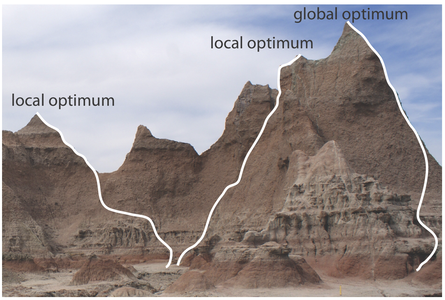
\(\newcommand{\avec}{\mathbf a}\) \(\newcommand{\bvec}{\mathbf b}\) \(\newcommand{\cvec}{\mathbf c}\) \(\newcommand{\dvec}{\mathbf d}\) \(\newcommand{\dtil}{\widetilde{\mathbf d}}\) \(\newcommand{\evec}{\mathbf e}\) \(\newcommand{\fvec}{\mathbf f}\) \(\newcommand{\nvec}{\mathbf n}\) \(\newcommand{\pvec}{\mathbf p}\) \(\newcommand{\qvec}{\mathbf q}\) \(\newcommand{\svec}{\mathbf s}\) \(\newcommand{\tvec}{\mathbf t}\) \(\newcommand{\uvec}{\mathbf u}\) \(\newcommand{\vvec}{\mathbf v}\) \(\newcommand{\wvec}{\mathbf w}\) \(\newcommand{\xvec}{\mathbf x}\) \(\newcommand{\yvec}{\mathbf y}\) \(\newcommand{\zvec}{\mathbf z}\) \(\newcommand{\rvec}{\mathbf r}\) \(\newcommand{\mvec}{\mathbf m}\) \(\newcommand{\zerovec}{\mathbf 0}\) \(\newcommand{\onevec}{\mathbf 1}\) \(\newcommand{\real}{\mathbb R}\) \(\newcommand{\twovec}[2]{\left[\begin{array}{r}#1 \\ #2 \end{array}\right]}\) \(\newcommand{\ctwovec}[2]{\left[\begin{array}{c}#1 \\ #2 \end{array}\right]}\) \(\newcommand{\threevec}[3]{\left[\begin{array}{r}#1 \\ #2 \\ #3 \end{array}\right]}\) \(\newcommand{\cthreevec}[3]{\left[\begin{array}{c}#1 \\ #2 \\ #3 \end{array}\right]}\) \(\newcommand{\fourvec}[4]{\left[\begin{array}{r}#1 \\ #2 \\ #3 \\ #4 \end{array}\right]}\) \(\newcommand{\cfourvec}[4]{\left[\begin{array}{c}#1 \\ #2 \\ #3 \\ #4 \end{array}\right]}\) \(\newcommand{\fivevec}[5]{\left[\begin{array}{r}#1 \\ #2 \\ #3 \\ #4 \\ #5 \\ \end{array}\right]}\) \(\newcommand{\cfivevec}[5]{\left[\begin{array}{c}#1 \\ #2 \\ #3 \\ #4 \\ #5 \\ \end{array}\right]}\) \(\newcommand{\mattwo}[4]{\left[\begin{array}{rr}#1 \amp #2 \\ #3 \amp #4 \\ \end{array}\right]}\) \(\newcommand{\laspan}[1]{\text{Span}\{#1\}}\) \(\newcommand{\bcal}{\cal B}\) \(\newcommand{\ccal}{\cal C}\) \(\newcommand{\scal}{\cal S}\) \(\newcommand{\wcal}{\cal W}\) \(\newcommand{\ecal}{\cal E}\) \(\newcommand{\coords}[2]{\left\{#1\right\}_{#2}}\) \(\newcommand{\gray}[1]{\color{gray}{#1}}\) \(\newcommand{\lgray}[1]{\color{lightgray}{#1}}\) \(\newcommand{\rank}{\operatorname{rank}}\) \(\newcommand{\row}{\text{Row}}\) \(\newcommand{\col}{\text{Col}}\) \(\renewcommand{\row}{\text{Row}}\) \(\newcommand{\nul}{\text{Nul}}\) \(\newcommand{\var}{\text{Var}}\) \(\newcommand{\corr}{\text{corr}}\) \(\newcommand{\len}[1]{\left|#1\right|}\) \(\newcommand{\bbar}{\overline{\bvec}}\) \(\newcommand{\bhat}{\widehat{\bvec}}\) \(\newcommand{\bperp}{\bvec^\perp}\) \(\newcommand{\xhat}{\widehat{\xvec}}\) \(\newcommand{\vhat}{\widehat{\vvec}}\) \(\newcommand{\uhat}{\widehat{\uvec}}\) \(\newcommand{\what}{\widehat{\wvec}}\) \(\newcommand{\Sighat}{\widehat{\Sigma}}\) \(\newcommand{\lt}{<}\) \(\newcommand{\gt}{>}\) \(\newcommand{\amp}{&}\) \(\definecolor{fillinmathshade}{gray}{0.9}\)Figure \(\PageIndex{1}\) shows a portion of the South Dakota Badlands, a barren landscape that includes many narrow ridges formed through erosion. Suppose you wish to climb to the highest point on this ridge. Because the shortest path to the summit is not obvious, you might adopt the following simple rule: look around you and take one step in the direction that has the greatest change in elevation, and then repeat until no further step is possible. The route you follow is the result of a systematic search that uses a searching algorithm. Of course there are as many possible routes as there are starting points, three examples of which are shown in Figure \(\PageIndex{1}\). Note that some routes do not reach the highest point—what we call the global optimum. Instead, many routes end at a local optimum from which further movement is impossible.
We can use a systematic searching algorithm to locate the optimum response. We begin by selecting an initial set of factor levels and measure the response. Next, we apply the rules of our searching algorithm to determine a new set of factor levels and measure its response, continuing this process until we reach an optimum response. Before we consider two common searching algorithms, let’s consider how we evaluate a searching algorithm.
Effectiveness and Efficiency
A searching algorithm is characterized by its effectiveness and its efficiency. To be effective, a searching algorithm must find the response surface’s global optimum, or at least reach a point near the global optimum. A searching algorithm may fail to find the global optimum for several reasons, including a poorly designed algorithm, uncertainty in measuring the response, and the presence of local optima. Let’s consider each of these potential problems.
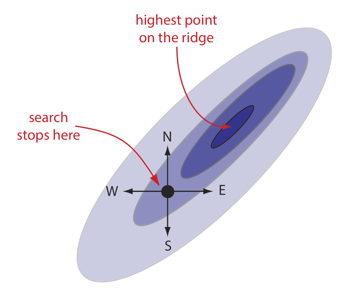
A poorly designed algorithm may prematurely end the search before it reaches the response surface’s global optimum. As shown in Figure \(\PageIndex{2}\), when you climb a ridge that slopes up to the northeast, an algorithm is likely to fail it if limits your steps only to the north, south, east, or west. An algorithm that cannot respond to a change in the direction of steepest ascent is not an effective algorithm.
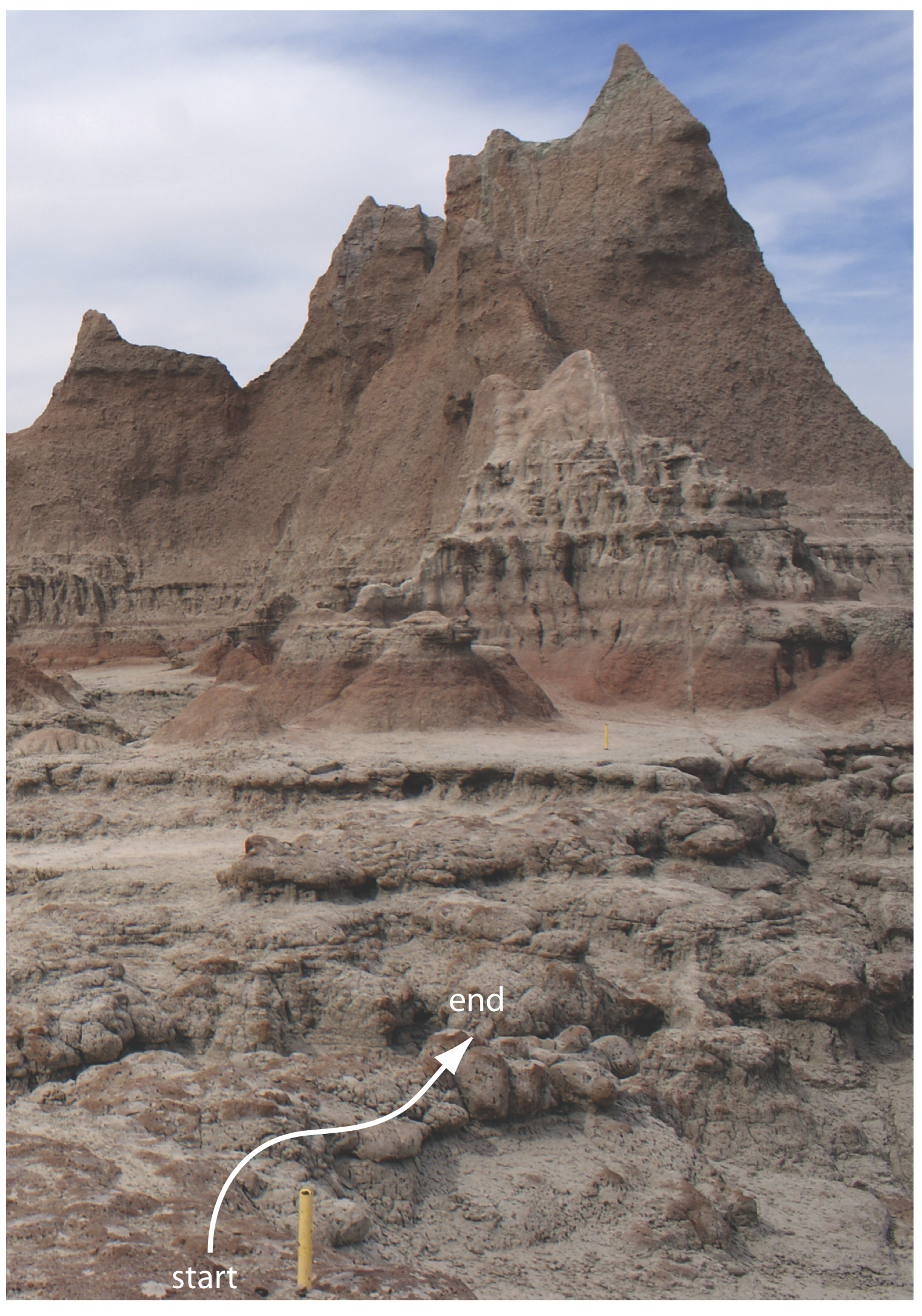
All measurements contain uncertainty, or noise, that affects our ability to characterize the underlying signal. When the noise is greater than the local change in the signal, then a searching algorithm is likely to end before it reaches the global optimum. Figure \(\PageIndex{3}\), which provides a different view of Figure \(\PageIndex{1}\), shows us that the relatively flat terrain leading up to the ridge is heavily weathered and very uneven. Because the variation in local height (the noise) exceeds the slope (the signal), our searching algorithm ends the first time we step up onto a less weathered local surface that is higher than the immediately surrounding surfaces.
Finally, a response surface may contain several local optima, only one of which is the global optimum. If we begin the search near a local optimum, our searching algorithm may never reach the global optimum. The ridge in Figure \(\PageIndex{1}\), for example, has many peaks. Only those searches that begin at the far right will reach the highest point on the ridge. Ideally, a searching algorithm should reach the global optimum regardless of where it starts.
A searching algorithm always reaches an optimum. Our problem, of course, is that we do not know if it is the global optimum. One method for evaluating a searching algorithm’s effectiveness is to use several sets of initial factor levels, find the optimum response for each, and compare the results. If we arrive at or near the same optimum response after starting from very different locations on the response surface, then we are more confident that is it the global optimum.
Efficiency is a searching algorithm’s second desirable characteristic. An efficient algorithm moves from the initial set of factor levels to the optimum response in as few steps as possible. In seeking the highest point on the ridge in Figure \(\PageIndex{3}\), we can increase the rate at which we approach the optimum by taking larger steps. If the step size is too large, however, the difference between the experimental optimum and the true optimum may be unacceptably large. One solution is to adjust the step size during the search, using larger steps at the beginning and smaller steps as we approach the global optimum.