24: 3D NMR
- Page ID
- 332829
\( \newcommand{\vecs}[1]{\overset { \scriptstyle \rightharpoonup} {\mathbf{#1}} } \)
\( \newcommand{\vecd}[1]{\overset{-\!-\!\rightharpoonup}{\vphantom{a}\smash {#1}}} \)
\( \newcommand{\dsum}{\displaystyle\sum\limits} \)
\( \newcommand{\dint}{\displaystyle\int\limits} \)
\( \newcommand{\dlim}{\displaystyle\lim\limits} \)
\( \newcommand{\id}{\mathrm{id}}\) \( \newcommand{\Span}{\mathrm{span}}\)
( \newcommand{\kernel}{\mathrm{null}\,}\) \( \newcommand{\range}{\mathrm{range}\,}\)
\( \newcommand{\RealPart}{\mathrm{Re}}\) \( \newcommand{\ImaginaryPart}{\mathrm{Im}}\)
\( \newcommand{\Argument}{\mathrm{Arg}}\) \( \newcommand{\norm}[1]{\| #1 \|}\)
\( \newcommand{\inner}[2]{\langle #1, #2 \rangle}\)
\( \newcommand{\Span}{\mathrm{span}}\)
\( \newcommand{\id}{\mathrm{id}}\)
\( \newcommand{\Span}{\mathrm{span}}\)
\( \newcommand{\kernel}{\mathrm{null}\,}\)
\( \newcommand{\range}{\mathrm{range}\,}\)
\( \newcommand{\RealPart}{\mathrm{Re}}\)
\( \newcommand{\ImaginaryPart}{\mathrm{Im}}\)
\( \newcommand{\Argument}{\mathrm{Arg}}\)
\( \newcommand{\norm}[1]{\| #1 \|}\)
\( \newcommand{\inner}[2]{\langle #1, #2 \rangle}\)
\( \newcommand{\Span}{\mathrm{span}}\) \( \newcommand{\AA}{\unicode[.8,0]{x212B}}\)
\( \newcommand{\vectorA}[1]{\vec{#1}} % arrow\)
\( \newcommand{\vectorAt}[1]{\vec{\text{#1}}} % arrow\)
\( \newcommand{\vectorB}[1]{\overset { \scriptstyle \rightharpoonup} {\mathbf{#1}} } \)
\( \newcommand{\vectorC}[1]{\textbf{#1}} \)
\( \newcommand{\vectorD}[1]{\overrightarrow{#1}} \)
\( \newcommand{\vectorDt}[1]{\overrightarrow{\text{#1}}} \)
\( \newcommand{\vectE}[1]{\overset{-\!-\!\rightharpoonup}{\vphantom{a}\smash{\mathbf {#1}}}} \)
\( \newcommand{\vecs}[1]{\overset { \scriptstyle \rightharpoonup} {\mathbf{#1}} } \)
\(\newcommand{\longvect}{\overrightarrow}\)
\( \newcommand{\vecd}[1]{\overset{-\!-\!\rightharpoonup}{\vphantom{a}\smash {#1}}} \)
\(\newcommand{\avec}{\mathbf a}\) \(\newcommand{\bvec}{\mathbf b}\) \(\newcommand{\cvec}{\mathbf c}\) \(\newcommand{\dvec}{\mathbf d}\) \(\newcommand{\dtil}{\widetilde{\mathbf d}}\) \(\newcommand{\evec}{\mathbf e}\) \(\newcommand{\fvec}{\mathbf f}\) \(\newcommand{\nvec}{\mathbf n}\) \(\newcommand{\pvec}{\mathbf p}\) \(\newcommand{\qvec}{\mathbf q}\) \(\newcommand{\svec}{\mathbf s}\) \(\newcommand{\tvec}{\mathbf t}\) \(\newcommand{\uvec}{\mathbf u}\) \(\newcommand{\vvec}{\mathbf v}\) \(\newcommand{\wvec}{\mathbf w}\) \(\newcommand{\xvec}{\mathbf x}\) \(\newcommand{\yvec}{\mathbf y}\) \(\newcommand{\zvec}{\mathbf z}\) \(\newcommand{\rvec}{\mathbf r}\) \(\newcommand{\mvec}{\mathbf m}\) \(\newcommand{\zerovec}{\mathbf 0}\) \(\newcommand{\onevec}{\mathbf 1}\) \(\newcommand{\real}{\mathbb R}\) \(\newcommand{\twovec}[2]{\left[\begin{array}{r}#1 \\ #2 \end{array}\right]}\) \(\newcommand{\ctwovec}[2]{\left[\begin{array}{c}#1 \\ #2 \end{array}\right]}\) \(\newcommand{\threevec}[3]{\left[\begin{array}{r}#1 \\ #2 \\ #3 \end{array}\right]}\) \(\newcommand{\cthreevec}[3]{\left[\begin{array}{c}#1 \\ #2 \\ #3 \end{array}\right]}\) \(\newcommand{\fourvec}[4]{\left[\begin{array}{r}#1 \\ #2 \\ #3 \\ #4 \end{array}\right]}\) \(\newcommand{\cfourvec}[4]{\left[\begin{array}{c}#1 \\ #2 \\ #3 \\ #4 \end{array}\right]}\) \(\newcommand{\fivevec}[5]{\left[\begin{array}{r}#1 \\ #2 \\ #3 \\ #4 \\ #5 \\ \end{array}\right]}\) \(\newcommand{\cfivevec}[5]{\left[\begin{array}{c}#1 \\ #2 \\ #3 \\ #4 \\ #5 \\ \end{array}\right]}\) \(\newcommand{\mattwo}[4]{\left[\begin{array}{rr}#1 \amp #2 \\ #3 \amp #4 \\ \end{array}\right]}\) \(\newcommand{\laspan}[1]{\text{Span}\{#1\}}\) \(\newcommand{\bcal}{\cal B}\) \(\newcommand{\ccal}{\cal C}\) \(\newcommand{\scal}{\cal S}\) \(\newcommand{\wcal}{\cal W}\) \(\newcommand{\ecal}{\cal E}\) \(\newcommand{\coords}[2]{\left\{#1\right\}_{#2}}\) \(\newcommand{\gray}[1]{\color{gray}{#1}}\) \(\newcommand{\lgray}[1]{\color{lightgray}{#1}}\) \(\newcommand{\rank}{\operatorname{rank}}\) \(\newcommand{\row}{\text{Row}}\) \(\newcommand{\col}{\text{Col}}\) \(\renewcommand{\row}{\text{Row}}\) \(\newcommand{\nul}{\text{Nul}}\) \(\newcommand{\var}{\text{Var}}\) \(\newcommand{\corr}{\text{corr}}\) \(\newcommand{\len}[1]{\left|#1\right|}\) \(\newcommand{\bbar}{\overline{\bvec}}\) \(\newcommand{\bhat}{\widehat{\bvec}}\) \(\newcommand{\bperp}{\bvec^\perp}\) \(\newcommand{\xhat}{\widehat{\xvec}}\) \(\newcommand{\vhat}{\widehat{\vvec}}\) \(\newcommand{\uhat}{\widehat{\uvec}}\) \(\newcommand{\what}{\widehat{\wvec}}\) \(\newcommand{\Sighat}{\widehat{\Sigma}}\) \(\newcommand{\lt}{<}\) \(\newcommand{\gt}{>}\) \(\newcommand{\amp}{&}\) \(\definecolor{fillinmathshade}{gray}{0.9}\)Triple resonance experiments (3D) are a set of multi-dimensional nuclear magnetic resonance spectroscopy (NMR) experiments that link three types of atomic nuclei, typically consisting of 1H, 15N and 13C. These experiments are often used to assign specific resonance signals to specific atoms in an isotopically enriched protein.
3D experiments are generally based upon 2D experiments. Then a correlation to a third nucleus is added in a third dimension.
* All spectra are either from SDBS (Japan National Institute of Advanced Industrial Science and Technology) or simulated.
HNCO for Protein Analysis
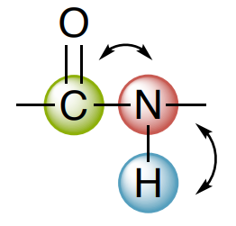
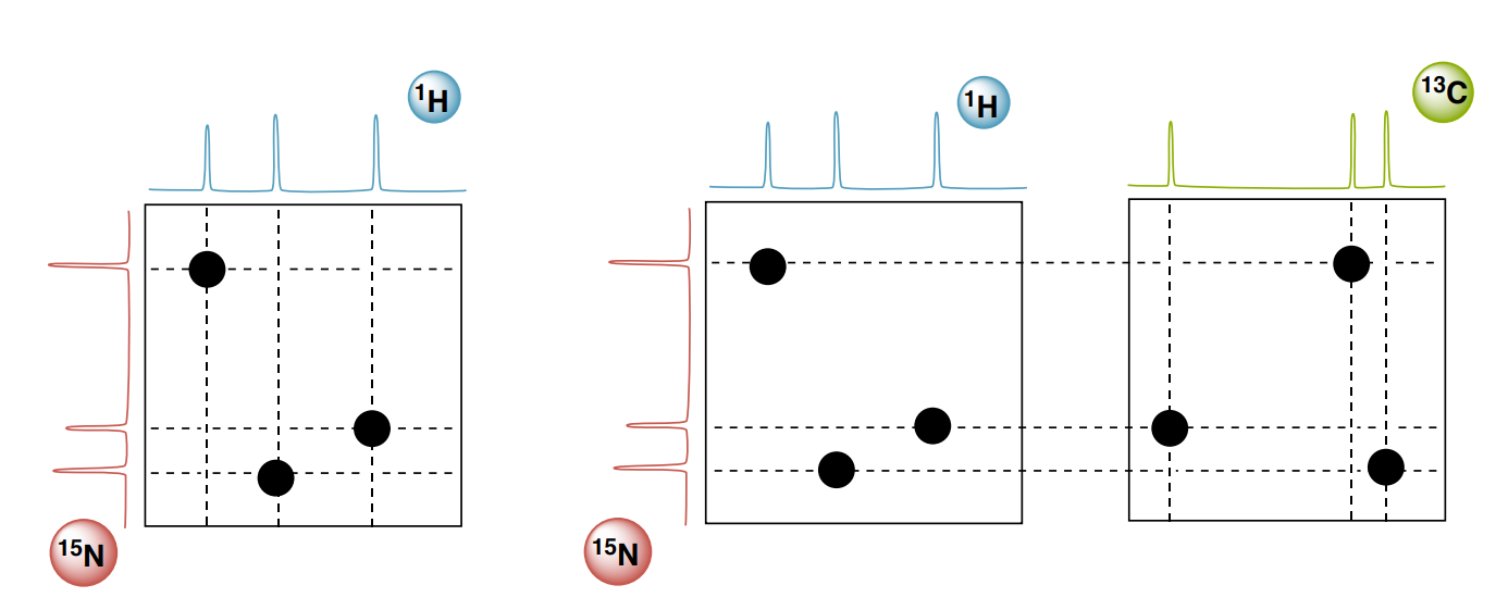
HNCO is based upon a 2D HSQC so the x and y axes are 1H and 15N, respectively. This is now extended into a third dimension that is a 13C dimension.
Each peak has 3 chemical shifts associated with it: HN, N, and CO and then correlations can then be used to determine the connections in a protein.
H-N Correlations
N-C Correlations
HNCACB and CBCA(CO)NH for Protein Backbone Analysis
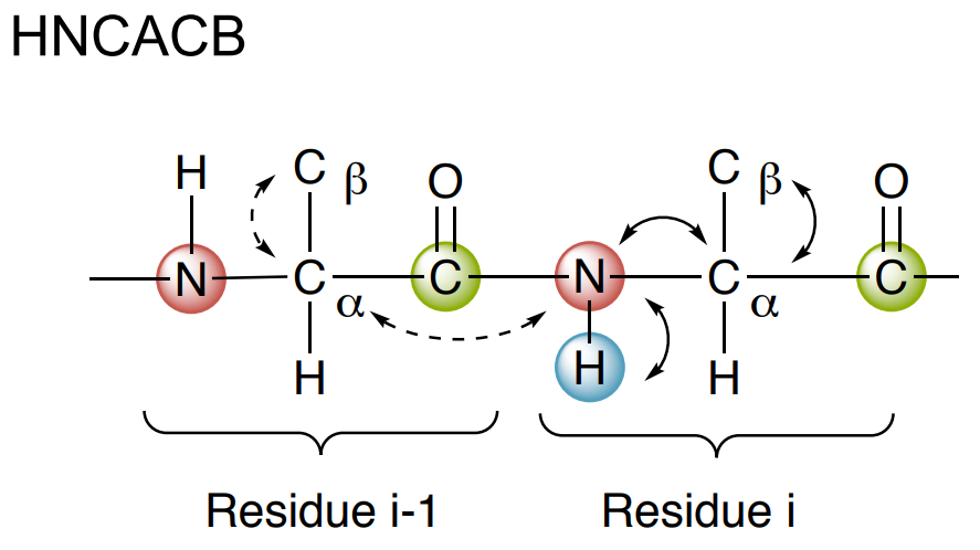
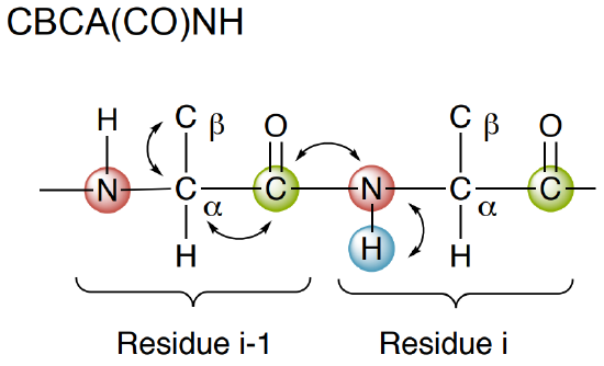
Standard triple resonance backbone assignment of proteins is based on two experiments: HNCACB and CBCA(CO)NH.
- The HNCACB correlates each NH group with the Cα and Cβ chemical shifts of its own residue (strongly) and of the residue preceding (weakly).
- The CBCA(CO)NH only correlates the NH group to the preceding Cα and Cβ chemical shifts.
- The HNCACB helps with ____________ (inter-residue, intra-residue, both) connections when determining backbone connections.
- The CBCA(CO)NH helps with ____________ (inter-residue, intra-residue, both) connections when determining backbone connections.
Strips for Analysis of 3D NMR
A common way of visualizing 3D spectra is strips.
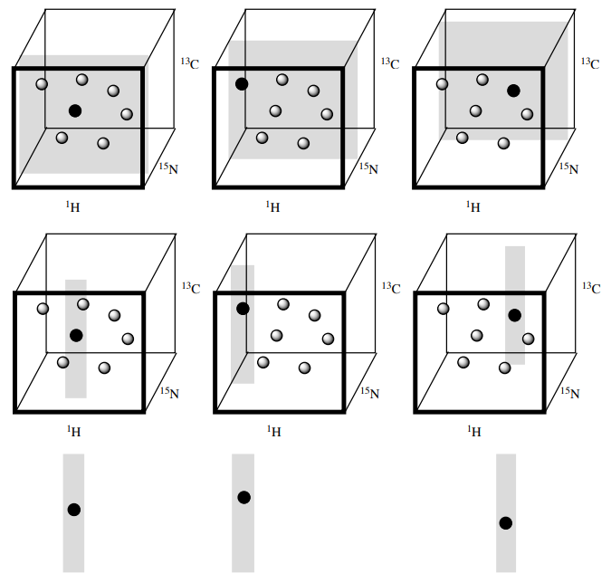
Consider, for instance, a particular z-plane of a 3D HNCO spectrum (a or b): you will probably end up with only one peak in that z-plane. You can trim the area you look at to the 1H region just surrounding your peak (c and d). This way you end up with a strip.
This strip corresponds to a particular 1H and 15N part of the spectrum but shows the complete 13C width. You can then pick out strips for each HSQC peak and then lay them next to one another for easy comparison (e).
Steps for Assigning the Protein Backbone
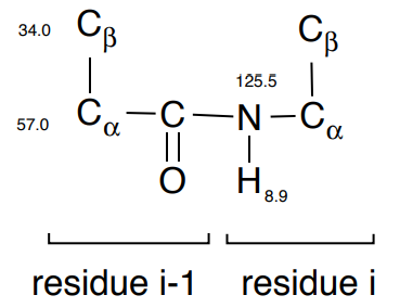
1. Identify one NH residue and find the correlations to the alpha (\(\alpha\)) carbon and beta (\(\beta\)) carbon using the \(\ce{C_{\beta} C_{\alpha}(CO)NH}\) experiment.
- Draw the correlations on the substructure:
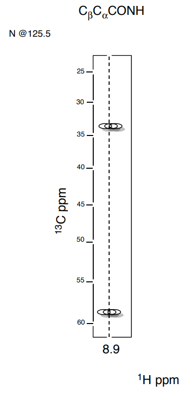
2. Repeat until all amide stretches (residue i) have been correlated to the \(\ce{C_{\beta} C_{\alpha}}\) on residues i-1.
Steps for Assigning the Protein Backbone (cont.)
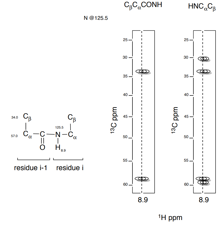
3. Next the \(\ce{C_{\beta} C_{\alpha}(CO)NH}\) can be correlated to the next \(\ce{C_{\beta} C_{\alpha}}\) sequence.
- Add the shifts of the next \(\ce{C_{\beta} C_{\alpha}}\).
- Add the next set of correlation arrows to the substructure below.
Steps for Assigning the Protein Backbone (cont.)
4. Next, we look for the NH correlated to the next residue (i+1).
- Add the shifts of the next NH residue
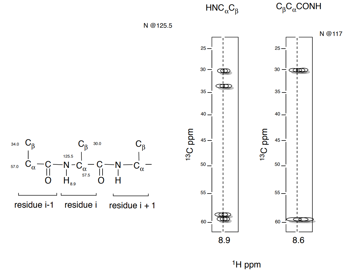
5. And then look for the next \(\ce{C_{\beta} C_{\alpha}}\) sequence.
- Add the shifts of the next Add the shifts of the next \(\ce{C_{\beta} C_{\alpha}}\) residue.
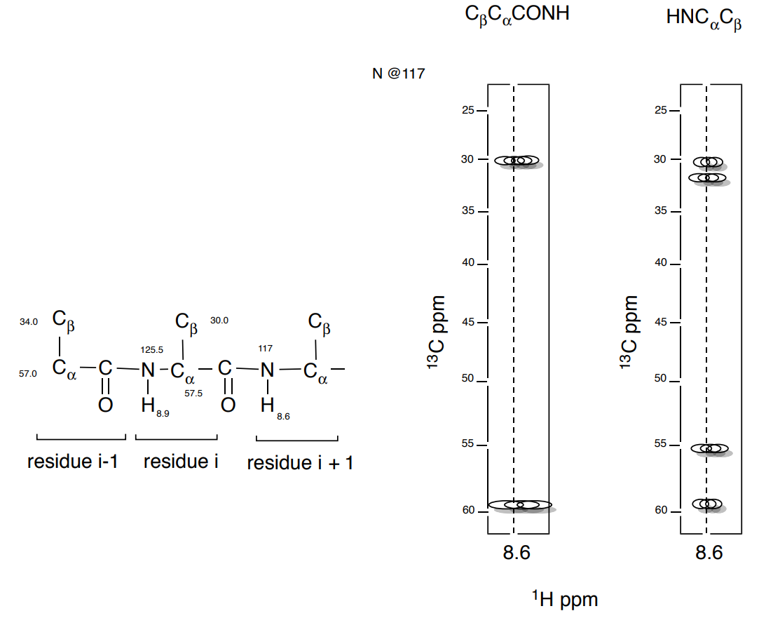
Steps for Assigning the Protein Backbone (cont.)
6. And repeat.
7. When you have finished this process, you will know the order in which the anonymous spin systems (HN/N/C/C) are arranged. However, we want to know the amino acid type to which each belongs.
a) Start by identifying those spin systems that have unique chemical shifts.
For example:
Gly: No \(\text{C}_{\beta}\) and \(\text{C}_{\alpha}\) ~ 45ppm
Ser/Thr: \(\text{C}_{\beta}\) is downfield of \(\text{C}_{\alpha}\) (~65-75ppm)
Ala: \(\text{C}_{\beta}\) is particularly upfield (~15-20ppm)
b) Consult Tables for standard shifts of amino acids:
8. For automated backbone assignment (NH, CO, Ca, Cb, Hb and Ha). It requires manually pick-peaking of 3D spectra for backbone assignment, such as CBCANH, CBCACONH etc.
9. There are more experiments to fully assign the side chains.
- TOCSY is often used for this process. Explain how this technique would be helpful.
Note: Practice Problems with Peptides using 3D NMR (and answers) are available at Graham, NMR2D [META: link missing]


