
Rovibrational Spectroscopy
- Page ID
- 1841
\( \newcommand{\vecs}[1]{\overset { \scriptstyle \rightharpoonup} {\mathbf{#1}} } \)
\( \newcommand{\vecd}[1]{\overset{-\!-\!\rightharpoonup}{\vphantom{a}\smash {#1}}} \)
\( \newcommand{\dsum}{\displaystyle\sum\limits} \)
\( \newcommand{\dint}{\displaystyle\int\limits} \)
\( \newcommand{\dlim}{\displaystyle\lim\limits} \)
\( \newcommand{\id}{\mathrm{id}}\) \( \newcommand{\Span}{\mathrm{span}}\)
( \newcommand{\kernel}{\mathrm{null}\,}\) \( \newcommand{\range}{\mathrm{range}\,}\)
\( \newcommand{\RealPart}{\mathrm{Re}}\) \( \newcommand{\ImaginaryPart}{\mathrm{Im}}\)
\( \newcommand{\Argument}{\mathrm{Arg}}\) \( \newcommand{\norm}[1]{\| #1 \|}\)
\( \newcommand{\inner}[2]{\langle #1, #2 \rangle}\)
\( \newcommand{\Span}{\mathrm{span}}\)
\( \newcommand{\id}{\mathrm{id}}\)
\( \newcommand{\Span}{\mathrm{span}}\)
\( \newcommand{\kernel}{\mathrm{null}\,}\)
\( \newcommand{\range}{\mathrm{range}\,}\)
\( \newcommand{\RealPart}{\mathrm{Re}}\)
\( \newcommand{\ImaginaryPart}{\mathrm{Im}}\)
\( \newcommand{\Argument}{\mathrm{Arg}}\)
\( \newcommand{\norm}[1]{\| #1 \|}\)
\( \newcommand{\inner}[2]{\langle #1, #2 \rangle}\)
\( \newcommand{\Span}{\mathrm{span}}\) \( \newcommand{\AA}{\unicode[.8,0]{x212B}}\)
\( \newcommand{\vectorA}[1]{\vec{#1}} % arrow\)
\( \newcommand{\vectorAt}[1]{\vec{\text{#1}}} % arrow\)
\( \newcommand{\vectorB}[1]{\overset { \scriptstyle \rightharpoonup} {\mathbf{#1}} } \)
\( \newcommand{\vectorC}[1]{\textbf{#1}} \)
\( \newcommand{\vectorD}[1]{\overrightarrow{#1}} \)
\( \newcommand{\vectorDt}[1]{\overrightarrow{\text{#1}}} \)
\( \newcommand{\vectE}[1]{\overset{-\!-\!\rightharpoonup}{\vphantom{a}\smash{\mathbf {#1}}}} \)
\( \newcommand{\vecs}[1]{\overset { \scriptstyle \rightharpoonup} {\mathbf{#1}} } \)
\(\newcommand{\longvect}{\overrightarrow}\)
\( \newcommand{\vecd}[1]{\overset{-\!-\!\rightharpoonup}{\vphantom{a}\smash {#1}}} \)
\(\newcommand{\avec}{\mathbf a}\) \(\newcommand{\bvec}{\mathbf b}\) \(\newcommand{\cvec}{\mathbf c}\) \(\newcommand{\dvec}{\mathbf d}\) \(\newcommand{\dtil}{\widetilde{\mathbf d}}\) \(\newcommand{\evec}{\mathbf e}\) \(\newcommand{\fvec}{\mathbf f}\) \(\newcommand{\nvec}{\mathbf n}\) \(\newcommand{\pvec}{\mathbf p}\) \(\newcommand{\qvec}{\mathbf q}\) \(\newcommand{\svec}{\mathbf s}\) \(\newcommand{\tvec}{\mathbf t}\) \(\newcommand{\uvec}{\mathbf u}\) \(\newcommand{\vvec}{\mathbf v}\) \(\newcommand{\wvec}{\mathbf w}\) \(\newcommand{\xvec}{\mathbf x}\) \(\newcommand{\yvec}{\mathbf y}\) \(\newcommand{\zvec}{\mathbf z}\) \(\newcommand{\rvec}{\mathbf r}\) \(\newcommand{\mvec}{\mathbf m}\) \(\newcommand{\zerovec}{\mathbf 0}\) \(\newcommand{\onevec}{\mathbf 1}\) \(\newcommand{\real}{\mathbb R}\) \(\newcommand{\twovec}[2]{\left[\begin{array}{r}#1 \\ #2 \end{array}\right]}\) \(\newcommand{\ctwovec}[2]{\left[\begin{array}{c}#1 \\ #2 \end{array}\right]}\) \(\newcommand{\threevec}[3]{\left[\begin{array}{r}#1 \\ #2 \\ #3 \end{array}\right]}\) \(\newcommand{\cthreevec}[3]{\left[\begin{array}{c}#1 \\ #2 \\ #3 \end{array}\right]}\) \(\newcommand{\fourvec}[4]{\left[\begin{array}{r}#1 \\ #2 \\ #3 \\ #4 \end{array}\right]}\) \(\newcommand{\cfourvec}[4]{\left[\begin{array}{c}#1 \\ #2 \\ #3 \\ #4 \end{array}\right]}\) \(\newcommand{\fivevec}[5]{\left[\begin{array}{r}#1 \\ #2 \\ #3 \\ #4 \\ #5 \\ \end{array}\right]}\) \(\newcommand{\cfivevec}[5]{\left[\begin{array}{c}#1 \\ #2 \\ #3 \\ #4 \\ #5 \\ \end{array}\right]}\) \(\newcommand{\mattwo}[4]{\left[\begin{array}{rr}#1 \amp #2 \\ #3 \amp #4 \\ \end{array}\right]}\) \(\newcommand{\laspan}[1]{\text{Span}\{#1\}}\) \(\newcommand{\bcal}{\cal B}\) \(\newcommand{\ccal}{\cal C}\) \(\newcommand{\scal}{\cal S}\) \(\newcommand{\wcal}{\cal W}\) \(\newcommand{\ecal}{\cal E}\) \(\newcommand{\coords}[2]{\left\{#1\right\}_{#2}}\) \(\newcommand{\gray}[1]{\color{gray}{#1}}\) \(\newcommand{\lgray}[1]{\color{lightgray}{#1}}\) \(\newcommand{\rank}{\operatorname{rank}}\) \(\newcommand{\row}{\text{Row}}\) \(\newcommand{\col}{\text{Col}}\) \(\renewcommand{\row}{\text{Row}}\) \(\newcommand{\nul}{\text{Nul}}\) \(\newcommand{\var}{\text{Var}}\) \(\newcommand{\corr}{\text{corr}}\) \(\newcommand{\len}[1]{\left|#1\right|}\) \(\newcommand{\bbar}{\overline{\bvec}}\) \(\newcommand{\bhat}{\widehat{\bvec}}\) \(\newcommand{\bperp}{\bvec^\perp}\) \(\newcommand{\xhat}{\widehat{\xvec}}\) \(\newcommand{\vhat}{\widehat{\vvec}}\) \(\newcommand{\uhat}{\widehat{\uvec}}\) \(\newcommand{\what}{\widehat{\wvec}}\) \(\newcommand{\Sighat}{\widehat{\Sigma}}\) \(\newcommand{\lt}{<}\) \(\newcommand{\gt}{>}\) \(\newcommand{\amp}{&}\) \(\definecolor{fillinmathshade}{gray}{0.9}\)In this section, we will learn how the rotational transitions of molecules can accompany the vibrational transitions. It is important to know how each peak correlates to the molecular processes of molecules. Rovibrational spectra can be analyzed to determine the average bond length.
Introduction
Each of the normal modes of vibration of heteronuclear diatomic molecules in the gas phase also contains closely-spaced (1-10 cm-1 difference) energy states attributable to rotational transitions that accompany the vibrational transitions. A molecule’s rotation can be affected by its vibrational transition because there is a change in bond length, so these rotational transitions are expected to occur. Since vibrational energy states are on the order of 1000 cm-1, the rotational energy states can be superimposed upon the vibrational energy states.
Selection Rules
Rotational and Vibration transitions (also known as rigid rotor and harmonic oscillator) of molecules help us identify how molecules interact with each other, their bond length as mentioned in the previous section. In order to know each transition, we have to consider other terms like wavenumber, force constant, quantum number, etc. There are rotational energy levels associated with all vibrational levels. From this, vibrational transitions can couple with rotational transitions to give rovibrational spectra. Rovibrational spectra can be analyzed to determine the average bond length.
We treat the molecule's vibrations as those of a harmonic oscillator (ignoring anharmonicity). The energy of a vibration is quantized in discrete levels and given by
\[E_v=h\nu \left(v+\dfrac{1}{2} \right) \nonumber \]
Where v is the vibrational quantum number and can have integer values 0, 1, 2..., and \(\nu\) is the frequency of the vibration given by:
\[\nu=\dfrac{1}{2\pi} \sqrt{ \dfrac{k}{\mu}} \nonumber \]
Where k is the force constant and \(\mu\) is the reduced mass of a diatomic molecule with atom masses m1 and m2, given by
\[\mu=\dfrac{{m}_1{m}_2}{{m}_1+{m}_2}\nonumber \]
We treat the molecule's rotations as those of a rigid rotor (ignoring centrifugal distortion). The energy of a rotation is also quantized in discrete levels given by
\[ E_r=\dfrac{h^2}{8\pi^2I} J(J+1)\nonumber \]
In which \(I\) is the moment of inertia, given by
\[{I}=\mu{r}^2\nonumber \]
where \(\mu\) is the reduced mass from above and r is the equilibrium bond length.
Experimentally, frequencies or wavenumbers are measured rather than energies, and dividing by h or hc gives more commonly seen term symbols, F(J) using the rotational quantum number \(J\) and the rotational constant \(B\) in either frequency
\[F(J)=\dfrac{E_r}{h}=\dfrac{h}{8\pi^2I} J(J+1)=BJ(J+1)\nonumber \]
or wavenumbers
\[F(J)=\dfrac{E_r}{hc}=\dfrac{h}{8\pi^2cI} J(J+1)=BJ(J+1)\nonumber \]
It is important to note in which units one is working since the rotational constant is always represented as \(B\), whether in frequency or wavenumbers.
Vibrational Transition Selection Rules
At room temperature, typically only the lowest energy vibrational state \(v= 0\) is populated, so typically \(v_0 = 0\) and \(∆v = +1\). The full selection rule is technically that \(∆v = ±1\), however here we assume energy can only go upwards because of the lack of population in the upper vibrational states.
Rotational Transition Selection Rules
At room temperature, states with \(J≠0\) can be populated since they represent the fine structure of vibrational states and have smaller energy differences than successive vibrational levels. Additionally, (∆J = ±1\) since a photon contains one quantum of angular momentum and we abide by the principle of conservation of energy. This is also the selection rule for rotational transitions.
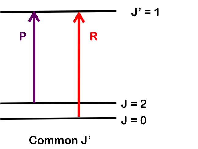
The transition \(∆J = 0\) (i.e. \(J" = 0\) and \(J' = 0\)), but where \(v_0 = 0\) and \(∆v = +1\), is forbidden and the pure vibrational transition is not observed in most cases. The rotational selection rule gives rise to an R-branch (when \(∆J = +1\)) and a P-branch (when \(∆J = -1\)). Each line of the branch is labeled \(R(J)\) or \(P(J)\), where \(J\) represents the value of the lower state.
R-branch
When \(∆J = +1\), i.e. the rotational quantum number in the ground state is one more than the rotational quantum number in the excited state – R branch (in French, riche or rich). To find the energy of a line of the R-branch:
\[ \begin{align*} \Delta{E} &=h\nu_0 +hB \left [J(J+1)-J^\prime (J^\prime{+1}) \right] \\[4pt] &=h\nu_0 +hB \left[(J+1)(J+2)-J(J+1)\right] \\[4pt] &=h\nu_0 +2hB(J+1) \end{align*} \]
P-branch
When \(∆J = -1\), i.e. the rotational quantum number in the ground state is one less than the rotational quantum number in the excited state – P branch (in French, pauvre or poor). To find the energy of a line of the P-branch:
\[ \begin{align*} \Delta{E} &=h\nu_0 +hB \left [J(J+1)-J^\prime(J^\prime+1) \right] \\[4pt] &=h\nu_0 +hB \left [J(J-1)-J(J+1) \right] \\[4pt] &=h\nu_0 -2hBJ \end{align*} \]
Q-branch
When \(∆J = 0\), i.e. the rotational quantum number in the ground state is the same as the rotational quantum number in the excited state – Q branch (simple, the letter between P and R). To find the energy of a line of the Q-branch:
\[ \begin{align*} \Delta{E} &= h\nu_0 +hB[J(J+1)-J^\prime(J^\prime+1)] \\[4pt] &=h\nu_0 \end{align*} \]
The Q-branch can be observed in polyatomic molecules and diatomic molecules with electronic angular momentum in the ground electronic state, e.g. nitric oxide, NO. Most diatomics, such as O2, have a small moment of inertia and thus very small angular momentum and yield no Q-branch.
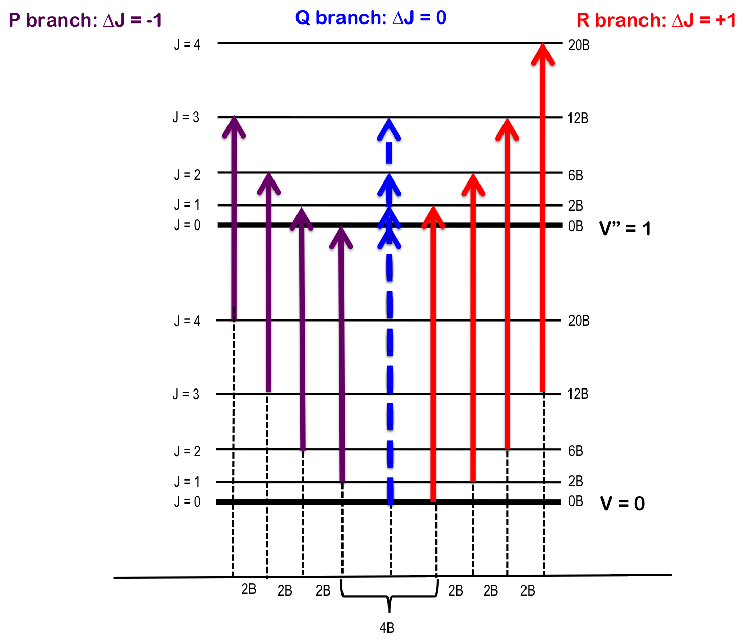
As seen in Figure 1, the lines of the P-branch (represented by purple arrows) and R-branch (represented by red arrows) are separated by specific multiples of B (2B), thus the bond length can be deduced without the need for pure rotational spectroscopy.
Energy
The total nuclear energy of the combined rotation-vibration terms, \(S(v, J)\), can be written as the sum of the vibrational energy and the rotational energy
\[ S(v,J)=G(v)+F(J) \nonumber \]
Where \(G(v)\) represents the energy of the harmonic oscillator, ignoring anharmonic components and \(S(J)\) represents the energy of a rigid rotor, ignoring centrifugal distortion. From this, we can derive
\[ S(v,J)=\nu_0 v+\dfrac{1}{2}+BJ(J+1)\nonumber \]
The relative intensity of the P- and R-branch lines depends on the thermal distribution of electrons; more specifically, they depend on the population of the lower \(J\) state. If we represent the population of the Jth upper level as NJ and the population of the lower state as N0, we can find the population of the upper state relative to the lower state using the Boltzmann distribution:
\[\dfrac{N_J}{N_0}={(2J+1)e}^{-E_r/kT}\nonumber \]
(2J+1) gives the degeneracy of the Jth upper level arising from the allowed values of \(M_J\) (+J to –J). As J increases, the degeneracy factor increases and the exponential factor decreases until at high J, the exponential factor wins out and NJ/N0 approaches zero at a certain level, Jmax. Thus, when
\[ \dfrac{d}{dJ} \left( \dfrac{N_J}{N_0} \right)=0\nonumber \]
by differentiation, we obtain
\[J_{max}=\left(\dfrac{kT}{2hcB}\right)^\frac{1}{2}-\dfrac{1}{2}\nonumber \]
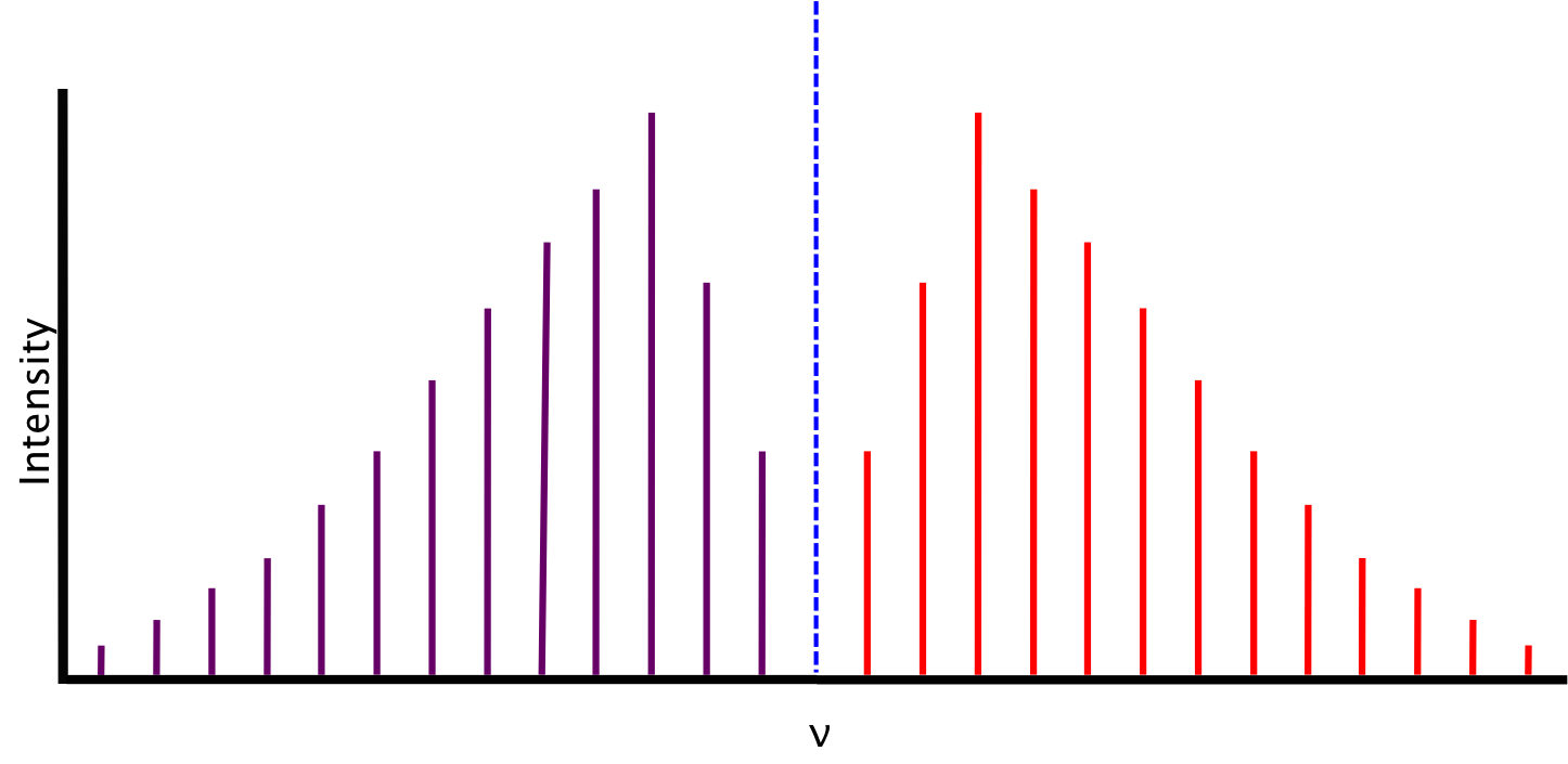
This is the reason that rovibrational spectral lines increase in energy to a maximum as J increases, then decrease to zero as J continues to increase, as seen in Figure 2 and Figure 3.
From this relationship, we can also deduce that in heavier molecules, B will decrease because the moment of inertia will increase, and the decrease in the exponential factor is less pronounced. This results in the population distribution shifting to higher values of J. Similarly, as temperature increases, the population distribution will shift towards higher values of J.
Ideal Spectrum
The spectrum we expect, based on the conditions described above, consists of lines equidistant in energy from one another, separated by a value of 2B. The relative intensity of the lines is a function of the rotational populations of the ground states, i.e. the intensity is proportional to the number of molecules that have made the transition. The overall intensity of the lines depends on the vibrational transition dipole moment.
Between P(1) and R(0) lies the zero gap, where the the first lines of both the P- and R-branch are separated by 4B, assuming that the rotational constant B is equal for both energy levels. The zero gap is also where we would expect the Q-branch, depicted as the dotted line, if it is allowed.
Real Spectra
We find that real spectra do not exactly fit the expectations from above.
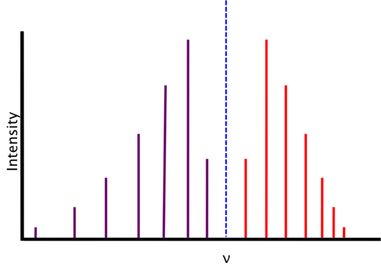
As energy increases, the R-branch lines become increasingly similar in energy (i.e., the lines move closer together) and as energy decreases, the P-branch lines become increasingly dissimilar in energy (i.e. the lines move farther apart). This is attributable to two phenomena: rotational-vibrational coupling and centrifugal distortion.
Rotational-Vibrational Coupling
As a diatomic molecule vibrates, its bond length changes. Since the moment of inertia is dependent on the bond length, it too changes and, in turn, changes the rotational constant B. We assumed above that \(B\) of \(R(0)\) and \(B\) of \(P(1)\) were equal, however they differ because of this phenomenon and \(B\) is given by
\[B_e= \left(-\alpha_e \nu+\dfrac{1}{2}\right)\nonumber \]
Where \({B}_{e}\) is the rotational constant for a rigid rotor and \(\alpha_{e}\) is the rotational-vibrational coupling constant. The information in the band can be used to determine B0 and B1 of the two different energy states as well as the rotational-vibrational coupling constant, which can be found by the method of combination differences.
Combination differences involves finding the values of B0 and B1 rotational-vibrational coupling constant by measuring the change for two different transitions sharing a common state.
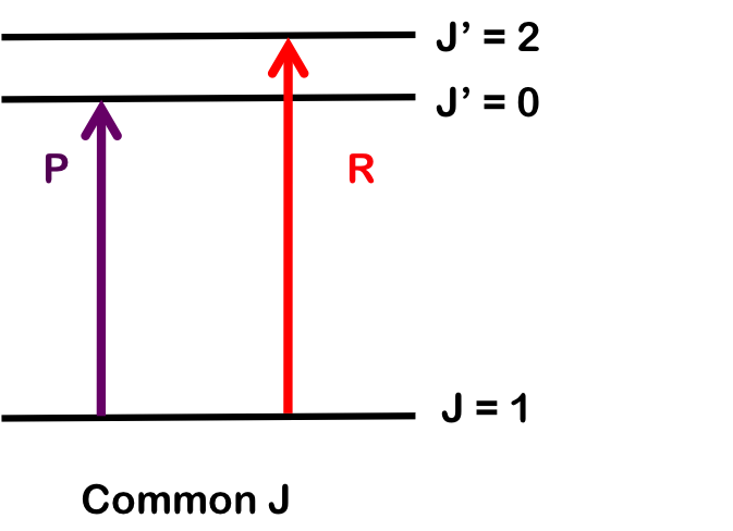
To determine \(B_1\), we pair transitions sharing a common lower state; here, R(1) and P(1). Note that the vibrational level does not change. Both branches begin with \(J = 1\), so by finding the difference in energy between the lines, we find \(B_1\).
\[\Delta E_R-\Delta E_P = E(\nu=1, J' =J+1) - E(\nu=1,J' =J-1)\nonumber \]
Inserting this information into the equation from above, we obtain
\[\begin{align*} &=\tilde{\nu} [R(J-1)]-\tilde{\nu} [P(J+1)] \\[4pt] &=\omega_0+B_1 (J+1)(J+2)-B_0 J(J+1) - \omega_0 -B_1(J-1)J + B_0 J(J+1) \\[4pt] &={4B}_1 \left(J+\dfrac{1}{2} \right)\end{align*} \]
If we plot \(\Delta E_R-\Delta E_P \) against \( J+ \dfrac{1}{2} \), we obtain a straight line with slope \(4B_1\).
Similarly, we can determine \(B_0\) by finding wavenumber differences in transitions sharing a common upper state; here, R(0) and P(2). Both branches terminate at \(J=1\) and differences will only depend on \(B_0\).
\[\begin{align*} &=\tilde {\nu} [R(J-1)]- \tilde{\nu} [P(J+1)] \\[4pt] &=\omega_0+B_1 J(J+1)-B_0 J(J-1)- \omega_0-B_1J(J+1)+B_0 (J+1)(J+2) \\[4pt] &={4B}_0{(J+}\dfrac{1}{2}{)} \end{align*}\]
As before, if we plot \(\Delta{E}_{R}-\Delta{E}_{P}\nonumber \) vs. \({(J+}\dfrac{1}{2}{)}\nonumber \), we obtain a straight line with slope \(4B_0\).
Following from this, we can obtain the rotational-vibrational coupling constant:
\[\alpha_{e}=B_0-B_1\nonumber \]
Centrifugal Distortion
Similarly to rotational-vibrational coupling, centrifugal distortion is related to the changing bond length of a molecule. A real molecule does not behave as a rigid rotor that has a rigid rod for a chemical bond, but rather acts as if it has a spring for a chemical bond. As the rotational velocity of a molecule increases, its bond length increases and its moment of inertia increases. As the moment of inertia increases, the rotational constant \(B\) decreases.
\[{F(J)=BJ(J+1)-DJ}^2{(J+1)}^2\nonumber \]
Where \(D\) is the centrifugal distortion constant and is related to the vibration wavenumber, \(\omega\)
\[D=\dfrac{4B^3}{\omega^2}\nonumber \]
When the above factors are accounted for, the actual energy of a rovibrational state is
\[ S(v,J)=\nu_0 v+\dfrac{1}{2}+B_e J (J+1)- \alpha_e \left(v+\dfrac{1}{2}\right) J(J+1)-D_e[J(J+1)]^2\nonumber \]
Find the reduced mass of D35Cl in kg, if the mass of D-2 is 2.014 amu and the mass of Cl-35 is 34.968 amu.
- Answer
-
\[\dfrac{2.014 amu \times 34.968 amu}{2.014 amu + 34.968 amu} = 1.807 ~amu\]
To convert to kg, multiple by 1.66 x 10⁻²⁷ kg/amu.
Answer: 3.00 x 10⁻²⁷ kg
Using information found in problem 1, calculate the rotational constant B (in wavenumbers) of D35Cl given that the average bond length is 1.2745 Å.
- Answer
-
We know that in wavenumbers, \(B=\dfrac{h}{8\pi^2cI}\).
First, we must solve for the moment of inertia, \(I\), using
\[{I}=\mu{r}^2=(3.00*10^{-27} kg)(1.2745 \times 10^{-10}m)^2\nonumber \] = 4.87 x 10-47 kg•m2= I
We can now substitute into the original formula to solve for B. h is Planck's constant, c is the speed of light in m/s and I = 4.87 x 10-47 kg•m2. This will give us the answer in m-1, then we can convert to cm-1.
Answer: 5.74 cm-1.
Using the rigid rotor approximation, estimate the bond length in a 12C16O molecule if the energy difference between J=1 and J=3 were to equal 14,234 cm-1.
- Answer
-
We use the same formula as above and expand the moment of inertia in order to solve for the average bond length.
\[B=\dfrac{h}{8\pi^2 c\mu r^2}\nonumber \]
We can deduce the rotational constant \(B\) since we know the distance between two energy states and the relationship
\[F(J)=BJ(J+1)\nonumber \]
The distance between \(J=1\) and \(J=3\) is \(10B\), so using the fact that B = 14,234 cm-1, B=1423.4 cm-1. We convert this to m-1 so that it will match up with the units of the speed of light (m/s) and obtain B = 142340 m-1.
Using the reduced mass formula, we find that µ = 1.138 x 10⁻²⁶ kg.
Answer: r = 81 Å.
References
- Hollas, M. J. Modern spectroscopy. (3rd ed.). Chichester: John Wiley & Sons, 1996.
- Hollas, M. J. Basic atomic and molecular spectroscopy. Cambridge: The Royal Society of Chemistry, 2002.
- Herzberg, G. Molecular spectra and molecular structure. (2nd ed.). New York: Prentice-Hall, 1950.
- Fetterolf, Monty L. Enhanced Intensity Distribution Analysis of the Rotational–Vibrational Spectrum of HCl. J. Chem. Ed. 2007, 84, 1064. DOI: 10.1021/ed084p1062