5.2: Relating Pressure, Volume, Amount, and Temperature - The Ideal Gas Law

Learning Objectives

• Identify the mathematical relationships between the various properties of gases
• Use the ideal gas law, and related gas laws, to compute the values of various gas properties under specified conditions

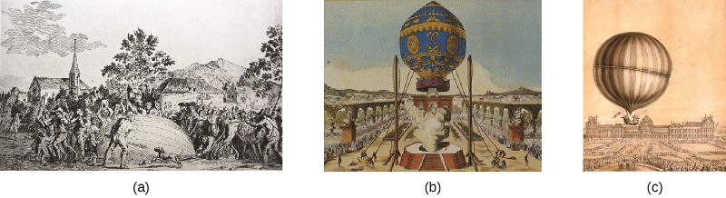
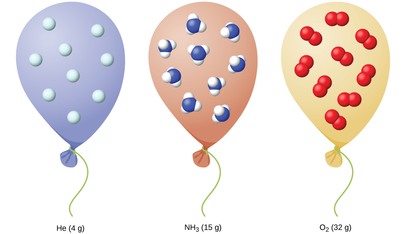
During the seventeenth and especially eighteenth centuries, driven both by a desire to understand nature and a quest to make balloons in which they could fly (Figure \(\PageIndex{1}\)), a number of scientists established the relationships between the macroscopic physical properties of gases, that is, pressure, volume, temperature, and amount of gas. Although their measurements were not precise by today’s standards, they were able to determine the mathematical relationships between pairs of these variables (e.g., pressure and temperature, pressure and volume) that hold for an ideal gas—a hypothetical construct that real gases approximate under certain conditions. Eventually, these individual laws were combined into a single equation—the ideal gas law—that relates gas quantities for gases and is quite accurate for low pressures and moderate temperatures. We will consider the key developments in individual relationships (for pedagogical reasons not quite in historical order), then put them together in the ideal gas law.

Figure \(\PageIndex{1}\): In 1783, the first (a) hydrogen-filled balloon flight, (b) manned hot air balloon flight, and (c) manned hydrogen-filled balloon flight occurred. When the hydrogen-filled balloon depicted in (a) landed, the frightened villagers of Gonesse reportedly destroyed it with pitchforks and knives. The launch of the latter was reportedly viewed by 400,000 people in Paris.

Pressure and Temperature: Amontons’s Law

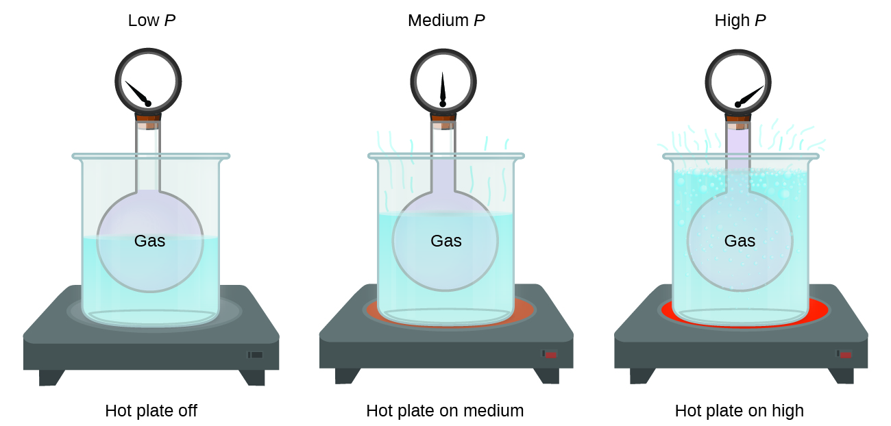
Imagine filling a rigid container attached to a pressure gauge with gas and then sealing the container so that no gas may escape. If the container is cooled, the gas inside likewise gets colder and its pressure is observed to decrease. Since the container is rigid and tightly sealed, both the volume and number of moles of gas remain constant. If we heat the sphere, the gas inside gets hotter (Figure \(\PageIndex{2}\)) and the pressure increases.

Figure \(\PageIndex{2}\): The effect of temperature on gas pressure: When the hot plate is off, the pressure of the gas in the sphere is relatively low. As the gas is heated, the pressure of the gas in the sphere increases.

This relationship between temperature and pressure is observed for any sample of gas confined to a constant volume. An example of experimental pressure-temperature data is shown for a sample of air under these conditions in Figure \(\PageIndex{3}\). We find that temperature and pressure are linearly related, and if the temperature is on the kelvin scale, then P and T are directly proportional (again, when volume and moles of gas are held constant); if the temperature on the kelvin scale increases by a certain factor, the gas pressure increases by the same factor.

Figure \(\PageIndex{3}\): For a constant volume and amount of air, the pressure and temperature are directly proportional, provided the temperature is in kelvin. (Measurements cannot be made at lower temperatures because of the condensation of the gas.) When this line is extrapolated to lower pressures, it reaches a pressure of 0 at –273 °C, which is 0 on the kelvin scale and the lowest possible temperature, called absolute zero.

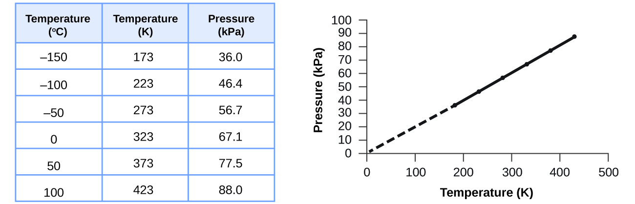
Guillaume Amontons was the first to empirically establish the relationship between the pressure and the temperature of a gas (~1700), and Joseph Louis Gay-Lussac determined the relationship more precisely (~1800). Because of this, the P-T relationship for gases is known as either Amontons’s law or Gay-Lussac’s law. Under either name, it states that the pressure of a given amount of gas is directly proportional to its temperature on the kelvin scale when the volume is held constant. Mathematically, this can be written:

\[P∝T\ce{\:or\:}P=\ce{constant}×T\ce{\:or\:}P=k×T \nonumber \]

where ∝ means “is proportional to,” and k is a proportionality constant that depends on the identity, amount, and volume of the gas.

For a confined, constant volume of gas, the ratio \(\dfrac{P}{T}\) is therefore constant (i.e., \(\dfrac{P}{T}=k\)). If the gas is initially in “Condition 1” (with P = P₁ and T = T₁), and then changes to “Condition 2” (with P = P₂ and T = T₂), we have that \(\dfrac{P_1}{T_1}=k\) and \(\dfrac{P_2}{T_2}=k\), which reduces to \(\dfrac{P_1}{T_1}=\dfrac{P_2}{T_2}\). This equation is useful for pressure-temperature calculations for a confined gas at constant volume. Note that temperatures must be on the kelvin scale for any gas law calculations (0 on the kelvin scale and the lowest possible temperature is called absolute zero). (Also note that there are at least three ways we can describe how the pressure of a gas changes as its temperature changes: We can use a table of values, a graph, or a mathematical equation.)

Example \(\PageIndex{1}\): Predicting Change in Pressure with Temperature

A can of hair spray is used until it is empty except for the propellant, isobutane gas.

1. On the can is the warning “Store only at temperatures below 120 °F (48.8 °C). Do not incinerate.” Why?
2. The gas in the can is initially at 24 °C and 360 kPa, and the can has a volume of 350 mL. If the can is left in a car that reaches 50 °C on a hot day, what is the new pressure in the can?

Solution

1. The can contains an amount of isobutane gas at a constant volume, so if the temperature is increased by heating, the pressure will increase proportionately. High temperature could lead to high pressure, causing the can to burst. (Also, isobutane is combustible, so incineration could cause the can to explode.)
2. We are looking for a pressure change due to a temperature change at constant volume, so we will use Amontons’s/Gay-Lussac’s law. Taking P₁ and T₁ as the initial values, T₂ as the temperature where the pressure is unknown and P₂ as the unknown pressure, and converting °C to K, we have:

\(\dfrac{P_1}{T_1}=\dfrac{P_2}{T_2}\textrm{ which means that }\dfrac{360\:\ce{kPa}}{297\:\ce K}=\dfrac{P_2}{323\:\ce K}\)

Rearranging and solving gives:

\(P_2=\mathrm{\dfrac{360\:kPa×323\cancel{K}}{297\cancel{K}}=390\:kPa}\)

Exercise \(\PageIndex{1}\)

A sample of nitrogen, N₂, occupies 45.0 mL at 27 °C and 600 torr. What pressure will it have if cooled to –73 °C while the volume remains constant?

Answer

400 torr

Query \(\PageIndex{1}\)

Volume and Temperature: Charles’s Law

If we fill a balloon with air and seal it, the balloon contains a specific amount of air at atmospheric pressure, let’s say 1 atm. If we put the balloon in a refrigerator, the gas inside gets cold and the balloon shrinks (although both the amount of gas and its pressure remain constant). If we make the balloon very cold, it will shrink a great deal, and it expands again when it warms up.

Video \(\PageIndex{1}\): This video shows how cooling and heating a gas causes its volume to decrease or increase, respectively.

These examples of the effect of temperature on the volume of a given amount of a confined gas at constant pressure are true in general: The volume increases as the temperature increases, and decreases as the temperature decreases. Volume-temperature data for a 1-mole sample of methane gas at 1 atm are listed and graphed in Figure \(\PageIndex{2}\).

Figuire \(\PageIndex{4}\): The volume and temperature are linearly related for 1 mole of methane gas at a constant pressure of 1 atm. If the temperature is in kelvin, volume and temperature are directly proportional. The line stops at 111 K because methane liquefies at this temperature; when extrapolated, it intersects the graph’s origin, representing a temperature of absolute zero.

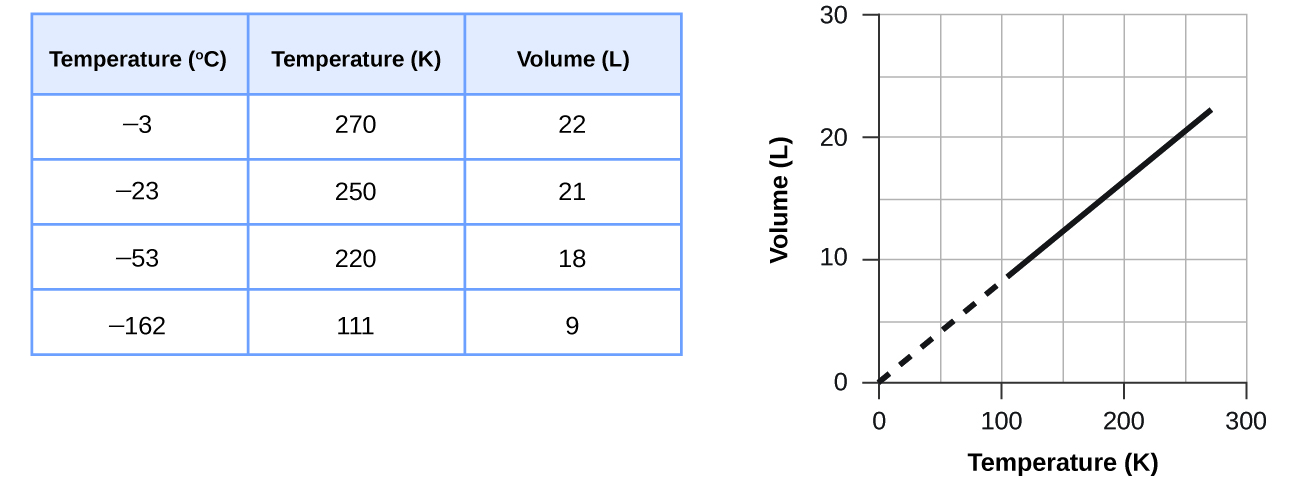
The relationship between the volume and temperature of a given amount of gas at constant pressure is known as Charles’s law in recognition of the French scientist and balloon flight pioneer Jacques Alexandre César Charles. Charles’s law states that the volume of a given amount of gas is directly proportional to its temperature on the kelvin scale when the pressure is held constant.

Mathematically, this can be written as:

\[VαT\ce{\:or\:}V=\ce{constant}·T\ce{\:or\:}V=k·T \nonumber \]

with k being a proportionality constant that depends on the amount and pressure of the gas.

For a confined, constant pressure gas sample, \(\dfrac{V}{T}\) is constant (i.e., the ratio = k), and as seen with the P-T relationship, this leads to another form of Charles’s law: \(\dfrac{V_1}{T_1}=\dfrac{V_2}{T_2}\).

Example \(\PageIndex{2}\): Predicting Change in Volume with Temperature

A sample of carbon dioxide, CO₂, occupies 0.300 L at 10 °C and 750 torr. What volume will the gas have at 30 °C and 750 torr?

Solution

Because we are looking for the volume change caused by a temperature change at constant pressure, this is a job for Charles’s law. Taking V₁ and T₁ as the initial values, T₂ as the temperature at which the volume is unknown and V₂ as the unknown volume, and converting °C into K we have:

\(\dfrac{V_1}{T_1}=\dfrac{V_2}{T_2}\textrm{ which means that }\dfrac{0.300\:\ce L}{283\:\ce K}=\dfrac{V_2}{303\:\ce K}\)

Rearranging and solving gives: \(V_2=\mathrm{\dfrac{0.300\:L×303\cancel{K}}{283\cancel{K}}=0.321\:L}\)

This answer supports our expectation from Charles’s law, namely, that raising the gas temperature (from 283 K to 303 K) at a constant pressure will yield an increase in its volume (from 0.300 L to 0.321 L).

Exercise \(\PageIndex{2}\)

A sample of oxygen, O₂, occupies 32.2 mL at 30 °C and 452 torr. What volume will it occupy at –70 °C and the same pressure?

Answer

21.6 mL

Example \(\PageIndex{3}\): Measuring Temperature with a Volume

Change Temperature is sometimes measured with a gas thermometer by observing the change in the volume of the gas as the temperature changes at constant pressure. The hydrogen in a particular hydrogen gas thermometer has a volume of 150.0 cm³ when immersed in a mixture of ice and water (0.00 °C). When immersed in boiling liquid ammonia, the volume of the hydrogen, at the same pressure, is 131.7 cm³. Find the temperature of boiling ammonia on the kelvin and Celsius scales.

Solution

A volume change caused by a temperature change at constant pressure means we should use Charles’s law. Taking V₁ and T₁ as the initial values, T₂ as the temperature at which the volume is unknown and V₂ as the unknown volume, and converting °C into K we have:

\[\dfrac{V_1}{T_1}=\dfrac{V_2}{T_2}\textrm{ which means that }\mathrm{\dfrac{150.0\:cm^3}{273.15\:K}}=\dfrac{131.7\:\ce{cm}^3}{T_2} \nonumber \]

Rearrangement gives \(T_2=\mathrm{\dfrac{131.7\cancel{cm}^3×273.15\:K}{150.0\:cm^3}=239.8\:K}\)

Subtracting 273.15 from 239.8 K, we find that the temperature of the boiling ammonia on the Celsius scale is –33.4 °C.

Exercise \(\PageIndex{3}\)

What is the volume of a sample of ethane at 467 K and 1.1 atm if it occupies 405 mL at 298 K and 1.1 atm?

Answer

635 mL

Query \(\PageIndex{1}\)

 

Charles’s Law: https://youtu.be/NBf510ZnlR0

Volume and Pressure: Boyle’s Law

If we partially fill an airtight syringe with air, the syringe contains a specific amount of air at constant temperature, say 25 °C. If we slowly push in the plunger while keeping temperature constant, the gas in the syringe is compressed into a smaller volume and its pressure increases; if we pull out the plunger, the volume increases and the pressure decreases. This example of the effect of volume on the pressure of a given amount of a confined gas is true in general. Decreasing the volume of a contained gas will increase its pressure, and increasing its volume will decrease its pressure. In fact, if the volume increases by a certain factor, the pressure decreases by the same factor, and vice versa. Volume-pressure data for an air sample at room temperature are graphed in Figure \(\PageIndex{5}\).

Figure \(\PageIndex{5}\): When a gas occupies a smaller volume, it exerts a higher pressure; when it occupies a larger volume, it exerts a lower pressure (assuming the amount of gas and the temperature do not change). Since P and V are inversely proportional, a graph of \(\dfrac{1}{P}\) vs. V is linear.

Unlike the P-T and V-T relationships, pressure and volume are not directly proportional to each other. Instead, \(P\) and \(V\) exhibit inverse proportionality: Increasing the pressure results in a decrease of the volume of the gas. Mathematically this can be written:

\[P \propto \dfrac{1}{V} \nonumber \]

or

\[P=k⋅ \dfrac{1}{V} \nonumber \]

or

\[PV=k \nonumber \]

or

\[P_1V_1=P_2V_2 \nonumber \]

with \(k\) being a constant. Graphically, this relationship is shown by the straight line that results when plotting the inverse of the pressure \(\left(\dfrac{1}{P}\right)\) versus the volume (V), or the inverse of volume \(\left(\dfrac{1}{V}\right)\) versus the pressure (\(P\)). Graphs with curved lines are difficult to read accurately at low or high values of the variables, and they are more difficult to use in fitting theoretical equations and parameters to experimental data. For those reasons, scientists often try to find a way to “linearize” their data. If we plot P versus V, we obtain a hyperbola (Figure \(\PageIndex{6}\)).

Figure \(\PageIndex{6}\): The relationship between pressure and volume is inversely proportional. (a) The graph of P vs. V is a hyperbola, whereas (b) the graph of \(\left(\dfrac{1}{P}\right)\) vs. V is linear.

The relationship between the volume and pressure of a given amount of gas at constant temperature was first published by the English natural philosopher Robert Boyle over 300 years ago. It is summarized in the statement now known as Boyle’s law: The volume of a given amount of gas held at constant temperature is inversely proportional to the pressure under which it is measured.

Example \(\PageIndex{4}\): Volume of a Gas Sample

The sample of gas has a volume of 15.0 mL at a pressure of 13.0 psi. Determine the pressure of the gas at a volume of 7.5 mL, using:

1. the P-V graph in Figure \(\PageIndex{6a}\)
2. the \(\dfrac{1}{P}\) vs. V graph in Figure \(\PageIndex{6b}\)
3. the Boyle’s law equation

Comment on the likely accuracy of each method.

Solution

1. Estimating from the P-V graph gives a value for P somewhere around 27 psi.
2. Estimating from the \(\dfrac{1}{P}\) versus V graph give a value of about 26 psi.
3. From Boyle’s law, we know that the product of pressure and volume (PV) for a given sample of gas at a constant temperature is always equal to the same value. Therefore we have P₁V₁ = k and P₂V₂ = k which means that P₁V₁ = P₂V₂.

Using P₁ and V₁ as the known values 13.0 psi and 15.0 mL, P₂ as the pressure at which the volume is unknown, and V₂ as the unknown volume, we have:

\[P_1V_1=P_2V_2\mathrm{\:or\:13.0\:psi×15.0\:mL}=P_2×7.5\:\ce{mL} \nonumber \]

Solving:

\[P_2=\mathrm{\dfrac{13.0\:psi×15.0\cancel{mL}}{7.5\cancel{mL}}=26\:psi} \nonumber \]

It was more difficult to estimate well from the P-V graph, so (a) is likely more inaccurate than (b) or (c). The calculation will be as accurate as the equation and measurements allow.

Exercise \(\PageIndex{4}\)

The sample of gas has a volume of 30.0 mL at a pressure of 6.5 psi. Determine the volume of the gas at a pressure of 11.0 psi, using:

1. the P-V graph in Figure \(\PageIndex{6a}\)
2. the \(\dfrac{1}{P}\) vs. V graph in Figure \(\PageIndex{6b}\)
3. the Boyle’s law equation

Comment on the likely accuracy of each method.

Answer a

about 17–18 mL

Answer b

~18 mL

Answer c

17.7 mL; it was more difficult to estimate well from the P-V graph, so (a) is likely more inaccurate than (b); the calculation will be as accurate as the equation and measurements allow

Breathing and Boyle’s Law

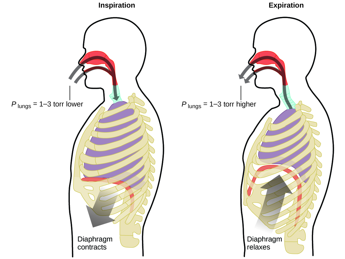
What do you do about 20 times per minute for your whole life, without break, and often without even being aware of it? The answer, of course, is respiration, or breathing. How does it work? It turns out that the gas laws apply here. Your lungs take in gas that your body needs (oxygen) and get rid of waste gas (carbon dioxide). Lungs are made of spongy, stretchy tissue that expands and contracts while you breathe. When you inhale, your diaphragm and intercostal muscles (the muscles between your ribs) contract, expanding your chest cavity and making your lung volume larger. The increase in volume leads to a decrease in pressure (Boyle’s law). This causes air to flow into the lungs (from high pressure to low pressure). When you exhale, the process reverses: Your diaphragm and rib muscles relax, your chest cavity contracts, and your lung volume decreases, causing the pressure to increase (Boyle’s law again), and air flows out of the lungs (from high pressure to low pressure). You then breathe in and out again, and again, repeating this Boyle’s law cycle for the rest of your life (Figure \(\PageIndex{7}\)).

Figure \(\PageIndex{7}\): Breathing occurs because expanding and contracting lung volume creates small pressure differences between your lungs and your surroundings, causing air to be drawn into and forced out of your lungs.

Boyle’s Law: https://youtu.be/lu86VSupPO4

Moles of Gas and Volume: Avogadro’s Law

The Italian scientist Amedeo Avogadro advanced a hypothesis in 1811 to account for the behavior of gases, stating that equal volumes of all gases, measured under the same conditions of temperature and pressure, contain the same number of molecules. Over time, this relationship was supported by many experimental observations as expressed by Avogadro’s law: For a confined gas, the volume (V) and number of moles (n) are directly proportional if the pressure and temperature both remain constant.

In equation form, this is written as:

\[V∝n\textrm{ or }V=k×n\textrm{ or }\dfrac{V_1}{n_1}=\dfrac{V_2}{n_2} \nonumber \]

Mathematical relationships can also be determined for the other variable pairs, such as P versus n, and n versus T.

Query \(\PageIndex{1}\)

Visit the PhET simulation below to investigate the relationships between pressure, volume, temperature, and amount of gas. Use the simulation to examine the effect of changing one parameter on another while holding the other parameters constant (as described in the preceding sections on the various gas laws).

Interactive Element

 

Avogadro’s Law: https://youtu.be/dRY3Trl4T24

Deriving the Ideal Gas Law

Any set of relationships between a single quantity (such as V) and several other variables (\(P\), \(T\), and \(n\)) can be combined into a single expression that describes all the relationships simultaneously. The three individual expressions are as follows:

• Boyle’s law

\[V \propto \dfrac{1}{P} \;\; \text{@ constant n and T}\]

• Charles’s law

\[V \propto T \;\; \text{@ constant n and P}\]

• Avogadro’s law

\[V \propto n \;\; \text{@ constant T and P}\]

Combining these three expressions gives

\[V \propto \dfrac{nT}{P} \tag{6.3.1}\]

which shows that the volume of a gas is proportional to the number of moles and the temperature and inversely proportional to the pressure. This expression can also be written as

\[V= {\rm Cons.} \left( \dfrac{nT}{P} \right) \tag{6.3.2}\]

By convention, the proportionality constant in Equation 6.3.1 is called the gas constant, which is represented by the letter \(R\). Inserting R into Equation 6.3.2 gives

\[ V = \dfrac{Rnt}{P} = \dfrac{nRT}{P} \tag{6.3.3}\]

Clearing the fractions by multiplying both sides of Equation 6.3.4 by \(P\) gives

\[PV = nRT \tag{6.3.4}\]

This equation is known as the ideal gas law.

An ideal gas is defined as a hypothetical gaseous substance whose behavior is independent of attractive and repulsive forces and can be completely described by the ideal gas law. In reality, there is no such thing as an ideal gas, but an ideal gas is a useful conceptual model that allows us to understand how gases respond to changing conditions. As we shall see, under many conditions, most real gases exhibit behavior that closely approximates that of an ideal gas. The ideal gas law can therefore be used to predict the behavior of real gases under most conditions. The ideal gas law does not work well at very low temperatures or very high pressures, where deviations from ideal behavior are most commonly observed.

Note

Significant deviations from ideal gas behavior commonly occur at low temperatures and very high pressures.

Before we can use the ideal gas law, however, we need to know the value of the gas constant R. Its form depends on the units used for the other quantities in the expression. If V is expressed in liters (L), P in atmospheres (atm), T in kelvins (K), and n in moles (mol), then

\[R = 0.08206 \dfrac{\rm L\cdot atm}{\rm K\cdot mol} \tag{6.3.5}\]

Because the product PV has the units of energy, R can also have units of J/(K•mol):

\[R = 8.3145 \dfrac{\rm J}{\rm K\cdot mol}\tag{6.3.6}\]

The ideal gas law is easy to remember and apply in solving problems, as long as you use the proper values and units for the gas constant, R.

Gases whose properties of P, V, and T are accurately described by the ideal gas law (or the other gas laws) are said to exhibit ideal behavior or to approximate the traits of an ideal gas. An ideal gas is a hypothetical construct that may be used along with kinetic molecular theory to effectively explain the gas laws as will be described in a later module of this chapter. Although all the calculations presented in this module assume ideal behavior, this assumption is only reasonable for gases under conditions of relatively low pressure and high temperature. In the final module of this chapter, a modified gas law will be introduced that accounts for the non-ideal behavior observed for many gases at relatively high pressures and low temperatures.

The ideal gas equation contains five terms, the gas constant R and the variable properties P, V, n, and T. Specifying any four of these terms will permit use of the ideal gas law to calculate the fifth term as demonstrated in the following example exercises.

Example \(\PageIndex{5}\): Using the Ideal Gas Law

Methane, CH₄, is being considered for use as an alternative automotive fuel to replace gasoline. One gallon of gasoline could be replaced by 655 g of CH₄. What is the volume of this much methane at 25 °C and 745 torr?

Solution

Exercise \(\PageIndex{5}\)

Calculate the pressure in bar of 2520 moles of hydrogen gas stored at 27 °C in the 180-L storage tank of a modern hydrogen-powered car.

Answer

350 bar

The Ideal Gas Law: https://youtu.be/rHGs23368mE

Query \(\PageIndex{1}\)

 

General Gas Equation

When a gas is described under two different conditions, the ideal gas equation must be applied twice - to an initial condition and a final condition. This is:

\[\begin{array}{cc}\text{Initial condition }(i) & \text{Final condition} (f)\\P_iV_i=n_iRT_i & P_fV_f=n_fRT_f\end{array}\]

Both equations can be rearranged to give:

\[R=\dfrac{P_iV_i}{n_iT_i} \hspace{1cm} R=\dfrac{P_fV_f}{n_fT_f}\]

The two equations are equal to each other since each is equal to the same constant \(R\). Therefore, we have:

\[\dfrac{P_iV_i}{n_iT_i}=\dfrac{P_fV_f}{n_fT_f}\tag{6.3.8}\]

The equation is called the general gas equation. The equation is particularly useful when one or two of the gas properties are held constant between the two conditions. In such cases, the equation can be simplified by eliminating these constant gas properties.

Example \(\PageIndex{6}\): Using the Combined Gas Law

Suppose that Charles had changed his plans and carried out his initial flight not in August but on a cold day in January, when the temperature at ground level was −10°C (14°F). How large a balloon would he have needed to contain the same amount of hydrogen gas at the same pressure as in Example \(\PageIndex{1}\)?

Given: temperature, pressure, amount, and volume in August; temperature in January

Asked for: volume in January

Strategy:

1. Use the results from Example \(\PageIndex{1}\) for August as the initial conditions and then calculate the change in volume due to the change in temperature from 30°C to −10°C. Begin by constructing a table showing the initial and final conditions.
2. Simplify the general gas equation by eliminating the quantities that are held constant between the initial and final conditions, in this case \(P\) and \(n\).
3. Solve for the unknown parameter.

Solution:

A To see exactly which parameters have changed and which are constant, prepare a table of the initial and final conditions:

Initial (August)	Final (January)
\(T_i=30\)°C = 303 K	\(T_f=\)​−10°C = 263 K
\(P_i=\)0.980 atm	\(P_f=\)0.980 atm
\(n_i=\)1.23 × 103 mol	\(n_f=\)1.23 × 103 mol
\(V_i=31150\) L	\(V_f=?\)

B Both \(n\) and \(P\) are the same in both cases​ (\(n_i=n_f,P_i=P_f\)). Therefore, Equation can be simplified to:

\[\dfrac{V_i}{T_i}=\dfrac{V_f}{T_f}\]

This is the relationship first noted by Charles.

C ​Solving the equation for \(V_f\), we get:

\[V_f=V_i\times\dfrac{T_f}{T_i}=\rm31150\;L\times\dfrac{263\;K}{303\;K}=2.70\times10^4\;L\]

It is important to check your answer to be sure that it makes sense, just in case you have accidentally inverted a quantity or multiplied rather than divided. In this case, the temperature of the gas decreases. Because we know that gas volume decreases with decreasing temperature, the final volume must be less than the initial volume, so the answer makes sense. We could have calculated the new volume by plugging all the given numbers into the ideal gas law, but it is generally much easier and faster to focus on only the quantities that change.

Exercise \(\PageIndex{6}\)

A sample of ammonia is found to occupy 0.250 L under laboratory conditions of 27 °C and 0.850 atm. Find the volume of this sample at 0 °C and 1.00 atm.

Answer

0.193 L

 

Query \(\PageIndex{1}\)

The Interdependence between Ocean Depth and Pressure in Scuba Diving

Whether scuba diving at the Great Barrier Reef in Australia (shown in Figure \(\PageIndex{9}\)) or in the Caribbean, divers must understand how pressure affects a number of issues related to their comfort and safety.

Figure \(\PageIndex{9}\): Scuba divers, whether at the Great Barrier Reef or in the Caribbean, must be aware of buoyancy, pressure equalization, and the amount of time they spend underwater, to avoid the risks associated with pressurized gases in the body. (credit: Kyle Taylor).

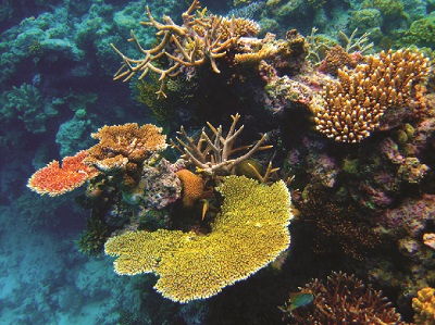
Pressure increases with ocean depth, and the pressure changes most rapidly as divers reach the surface. The pressure a diver experiences is the sum of all pressures above the diver (from the water and the air). Most pressure measurements are given in units of atmospheres, expressed as “atmospheres absolute” or ATA in the diving community: Every 33 feet of salt water represents 1 ATA of pressure in addition to 1 ATA of pressure from the atmosphere at sea level. As a diver descends, the increase in pressure causes the body’s air pockets in the ears and lungs to compress; on the ascent, the decrease in pressure causes these air pockets to expand, potentially rupturing eardrums or bursting the lungs. Divers must therefore undergo equalization by adding air to body airspaces on the descent by breathing normally and adding air to the mask by breathing out of the nose or adding air to the ears and sinuses by equalization techniques; the corollary is also true on ascent, divers must release air from the body to maintain equalization. Buoyancy, or the ability to control whether a diver sinks or floats, is controlled by the buoyancy compensator (BCD). If a diver is ascending, the air in his BCD expands because of lower pressure according to Boyle’s law (decreasing the pressure of gases increases the volume). The expanding air increases the buoyancy of the diver, and she or he begins to ascend. The diver must vent air from the BCD or risk an uncontrolled ascent that could rupture the lungs. In descending, the increased pressure causes the air in the BCD to compress and the diver sinks much more quickly; the diver must add air to the BCD or risk an uncontrolled descent, facing much higher pressures near the ocean floor. The pressure also impacts how long a diver can stay underwater before ascending. The deeper a diver dives, the more compressed the air that is breathed because of increased pressure: If a diver dives 33 feet, the pressure is 2 ATA and the air would be compressed to one-half of its original volume. The diver uses up available air twice as fast as at the surface.

Second Type of Ideal Gas Law Problems: https://youtu.be/WQDJOqddPI0

Standard Conditions of Temperature and Pressure

Scientists have chosen a particular set of conditions to use as a reference: 0°C (273.15 K) and \(\rm1\; bar = 100 \;kPa = 10^5\;Pa\) pressure, referred to as standard temperature and pressure (STP).

\[\text{STP:} \hspace{2cm} T=273.15\;{\rm K}\text{ and }P=\rm 1\;bar=10^5\;Pa\]

Please note that STP was defined differently in the past. The old definition was based on a standard pressure of 1 atm.

Figure \(\PageIndex{10}\): Since the number of moles in a given volume of gas varies with pressure and temperature changes, chemists use standard temperature and pressure (273.15 K and 1 atm or 101.325 kPa) to report properties of gases.

We can calculate the volume of 1.000 mol of an ideal gas under standard conditions using the variant of the ideal gas law given in Equation 6.3.4:

\[V=\dfrac{nRT}{P}\tag{6.3.7}\]

Thus the volume of 1 mol of an ideal gas is 22.71 L at STP and 22.41 L at 0°C and 1 atm, approximately equivalent to the volume of three basketballs. The molar volumes of several real gases at 0°C and 1 atm​ are given in Table 10.3, which shows that the deviations from ideal gas behavior are quite small. Thus the ideal gas law does a good job of approximating the behavior of real gases at 0°C and 1 atm​. The relationships described in Section 10.3 as Boyle’s, Charles’s, and Avogadro’s laws are simply special cases of the ideal gas law in which two of the four parameters (P, V, T, and n) are held fixed.

Table \(\PageIndex{1}\): Molar Volumes of Selected Gases at 0°C and 1 atm

Gas	Molar Volume (L)
He	22.434
Ar	22.397
H2	22.433
N2	22.402
O2	22.397
CO2	22.260
NH3	22.079

Summary

The behavior of gases can be described by several laws based on experimental observations of their properties. The pressure of a given amount of gas is directly proportional to its absolute temperature, provided that the volume does not change (Amontons’s law). The volume of a given gas sample is directly proportional to its absolute temperature at constant pressure (Charles’s law). The volume of a given amount of gas is inversely proportional to its pressure when temperature is held constant (Boyle’s law). Under the same conditions of temperature and pressure, equal volumes of all gases contain the same number of molecules (Avogadro’s law).

The equations describing these laws are special cases of the ideal gas law, PV = nRT, where P is the pressure of the gas, V is its volume, n is the number of moles of the gas, T is its kelvin temperature, and R is the ideal (universal) gas constant.

Key Equations

• PV = nRT

Summary

absolute zero

temperature at which the volume of a gas would be zero according to Charles’s law.

Amontons’s law

(also, Gay-Lussac’s law) pressure of a given number of moles of gas is directly proportional to its kelvin temperature when the volume is held constant

Avogadro’s law

volume of a gas at constant temperature and pressure is proportional to the number of gas molecules

Boyle’s law

volume of a given number of moles of gas held at constant temperature is inversely proportional to the pressure under which it is measured

Charles’s law

volume of a given number of moles of gas is directly proportional to its kelvin temperature when the pressure is held constant

ideal gas

hypothetical gas whose physical properties are perfectly described by the gas laws

ideal gas constant (R)

constant derived from the ideal gas equation R = 0.08226 L atm mol^–1 K^–1 or 8.314 L kPa mol^–1 K^–1

ideal gas law

relation between the pressure, volume, amount, and temperature of a gas under conditions derived by combination of the simple gas laws

standard conditions of temperature and pressure (STP)

273.15 K (0 °C) and 1 atm (101.325 kPa)

standard molar volume

volume of 1 mole of gas at STP, approximately 22.4 L for gases behaving ideally