6.2: Heteronuclear 3D NMR- Resonance Assignment in Proteins

In the previous Chapter we described 2D NMR spectroscopy, which offers significantly greater spectral resolution than basic 1D spectra. In this Chapter we will show how the well-resolved 2D ¹⁵N-HSQC resonances can be assigned to specific residues and chemical groups within protein samples. As an example, we will consider a couple of complementary types of 3D NMR data: HNCACB and CBCA(CO)NH and their joint application for making heteronuclear NMR resonance assignment in proteins. Such an assignment opens a number of ways to probe structure and function (e.g. ligand binding) for the target protein samples.

Learning Objectives

• Grasp why the resonance assignment of 2D ¹⁵N-HSQC can be beneficial : the case of ligand (drug) binding by a protein (therapeutic target)
• Familiarize with 3D heteronuclear through-bond (J-coupling) NMR : introduction and case of HNCACB and CBCA(CO)NH pair of 3D experiments
• Follow an example of assignment of heteronuclear NMR resonances (¹H_N, ¹⁵N_H, ¹³Cα, ¹³Cβ) from a combination of 2D ¹⁵N-HSQC and 3D HNCACB/CBCA(CO)NH

¹⁵N-HSQC as an assay for probing protein – ligand interactions: the need for the NMR resonance assignment

During the process of rational drug design, it is often necessary to characterize the interactions between the therapeutic target (protein) and candidate drug (ligand) beyond determination of the binding affinity (K_d). Heteronuclear solution NMR experiments ¹⁵N-HSQC can provide significant insight for such interactions. Let’s recall that most of the signals in this 2D NMR spectra originate from backbone H-N amide groups and some (minority) from the side chain NH and NH₂ groups. The position of ¹⁵N-HSQC resonances are defined by the ¹H_N and ¹⁵N_H chemical shift values, which in tern depend on the local electronic environment. Ligand binding changes such an environment for the residues forming the binding site even if the tertiary structure of the rest of the protein does not get perturbed. In such a case, the 15N-HSQC resonance pattern undergoes local changes: only the resonances representing NH groups involved in the binding site change their position significantly (>0.05 ppm in ¹H and/or >0.2 ppm in ¹⁵N dimension) or signal intensity (including peak disappearance). Figure VI.2.A illustrates such a change.

Figure VI.2.A ¹⁵N-HSQC as a method to characterize ligand (L) – target (T) interactions. In this case, the target is an ¹⁵N-labeled protein, the ligand has no ¹⁵N labeling. The target resonance labels do not convey any information about the resonance assignment (yet). Panel A shows the ¹⁵N-HSQC of the ¹⁵N-labeled target protein (T) in isolation. Panel B depicts ¹⁵N-HSQC of the ¹⁵N-labeled target protein (T) in presence of a substantial amount of the unlabeled ligand (L).

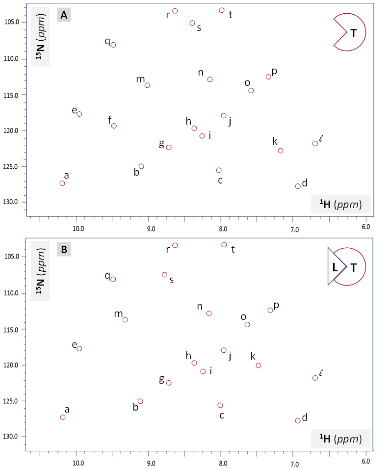
Importantly, every ¹⁵N-HSQC resonance in Figure VI.2.A is labeled with a single letter to help identify specific peaks which undergo spectral changes upon ligand binding. This data could have much greater impact if the peaks which underwent the most pronounced changes in position and/or intensity were assigned to specific amino acid residues within the polypeptide and chemical groups within those residues (backbone vs. side chain). The rest of this Chapter demonstrates some of the fundamentals of the heteronuclear NMR resonance assignment methodology.

Heteronuclear 3D NMR introduction: CBCA(CO)NH spectrum as an example

Just like every 2D 15N-HSQC resonance reports a J-coupling via a covalent bond between an 15N and 1H spin-½ nuclei, there are 3D NMR experiments which report resonances originating from J-coupling (through-bond) of three types of spin-½ nuclei (¹H, ¹³C, ¹⁵N). In this section we will introduce two such types of 3D NMR data: HNCAB and CBCA(CO)NH. In order to produce a protein sample with nearly complete uniform labeling with ¹³C and ¹⁵N isotopes, bacterial recombinant protein expression can be performed in a minimal media supplemented with ¹³C-labeled glucose and ¹⁵N-labeled ammonium chloride as the sole sources of carbon and nitrogen respectively. Figure VI.2.B introduces a general concept of a 3D NMR data and shows an element of 3D CBCA(CO)NH spectrum.

Figure VI.2.B An introduction into heteronuclear 3D NMR spectra in general and CBCA(CO)NH in particular. A: J-coupled spin systems involved into 3D CBCA(CO)NH through-bond resonance generation- backbone HN group of a residue and Cα and Cβ of a preceding residue. B: a schematic depiction of a heteronuclear (¹H, ¹³C, ¹⁵N) 3D NMR spectrum. C: a fragment of a single ¹⁵N plane showing two 3D resonances originating from J-coupling of the backbone amide group of residue j and Cα and Cβ nuclei of preceding residue j-1. The Figure design is courtesy of Heather Miears (the Smirnov lab, WWU, 2017).

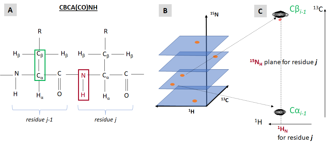
Each resonance (“cross-peak”) of a 3D CBCA(CO)NH spectrum indicates a through-bond (J-coupling scalar) interaction between two atoms of the backbone amide group (¹H_N and ¹⁵N_H) or residue j and Cα and Cβ nuclei (¹³C) of preceding residue j-1. The name of the experiment, CBCA(CO)NH refers to the specific spin-½ nuclei involved (and not involved) in relevant J-coupling interactions: Cβ and Cα are J-coupled to NH while the connecting carbonyl carbon is not reporting any NMR signal (although its magnetization state is affected during the experiment). Two types of residues generate special CBCA(CO)NH peak pattern: prolines have no amide proton, so they do not have CBCA(CO)NH peaks linked with their amide groups. Glycine residues have no Cβ, therefore for any residue following a glycine only a single CBCA(CO)NH resonance will be observed (from glycine NH to previous Cα).

The NMR resonance assignment: combined use of two complementary datasets HNCACB and CBCA(CO)NH

By itself, CBCA(CO)NH does not convey much of sequential information. Another heteronuclear 3D NMR dataset, HNCACB, affords a powerful complement here. Just like CBCA(CO)NH, HNCACB reports resonances originating from J-coupling between backbone amide group and Cα / Cβ nuclei. The difference is that HNCACN reports two additional peaks, all intra-residual: between HN and Cα a Cβ spins (Figure VI.2.C).

Figure VI.2.C Identical fragments of 1%N-planes from two complementary 3D NMR datasets. A: HNCACB and B: CBCA(CO)NH. The two CBCA(CO)NH resonances have exact HNCACB counterparts. In addition to those two peaks, HNCACB also has two more resonances originating from backbone HN grouped J-coupled with Cα and Cβ within the same residue. Importantly, two pairs of HNCACB resonances have the opposite signs: those involved Cα_j and Cα_j-1 are positive (black contours) and those involved Cβ_j and Cβ_j-1 are negative (red contours). All the four HNCACB and two CBCA(CO)NH peaks share the same ¹HN and ¹⁵NH chemical shift values since they originate from the same backbone amide of residue j. This combination of two related spectra and positive/negative HNCACB peak intensities allow unambiguous determination of the four carbon chemical shifts and their assignment to the current and previous residues. The Figure design is courtesy of Heather Miears (the Smirnov lab, WWU, 2017).

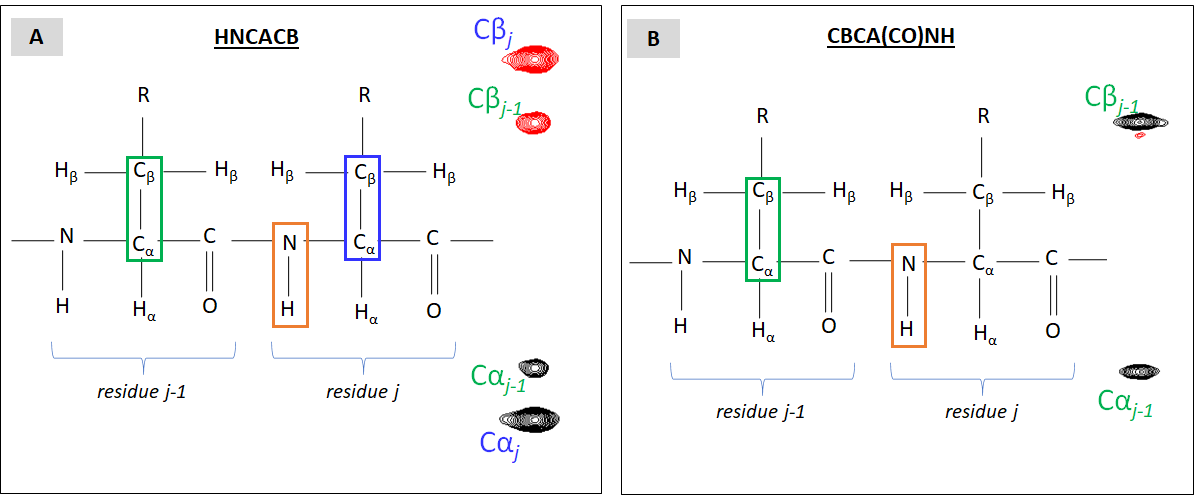
Typically, HNCACB and CBCA(CO)NH are acquired with identical parameters including spectral width in all three dimensions and the same number of data points in the ¹⁵N dimension (or ¹⁵N planes as on panel B of Figure VI.2.B) Now, let’s imagine that we go through every ¹⁵N plane and build the pairs of “residue j / residue j-1″ HNCAB/CBCA(CO)NH peaks. This does not give us the sequence-specific NMR resonance assignments yet but already creates such pairs of 3D cross-peaks linked to di-peptides within the sequence. Now, let’s take into account that for some types of residues their 13Cα and 13Cβ chemical shift values differs remarkably from those from other residue types. For details, take a look at BMRB chemical shift statistics for amino acid residues with emphasis on Gly, Ala, Ser, Thr. Knowing where such residues are positioned within the polypeptide sequence, we can start “connecting the dots” by mapping HNCACB/CBCA(CO)NH planes and di-peptides on actual amino acid sequence.

Figure VI.2.D An example of combined use of HNCACB and CBCA(CO)NH experiments for the backbone NMR resonance assignment in proteins. Cα and Cα labels are color coded: blue for intra-residual signals and green for preceding carbons (Cα-1, Cβ-1). HNCACB contours are color-coded: black for positive signals (Cα) and red for negative ones (Cβ). Asterisks (*) indicate resonances which originate from residues other than Alal46 (note that the ¹H_N chemical shift values for those peaks are different than for Alal46). The Figure design is courtesy of Heather Miears (the Smirnov lab, WWU, 2017).

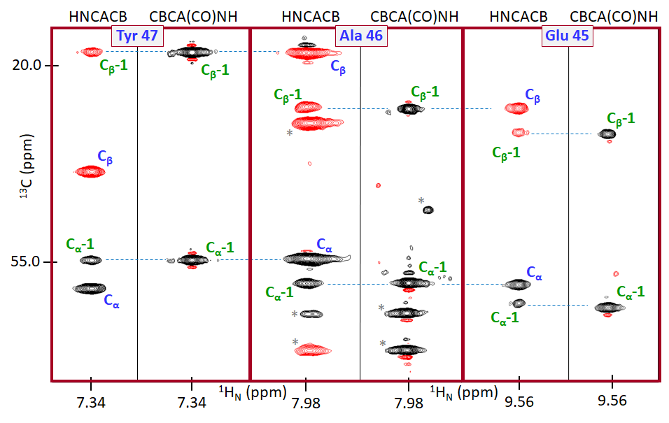
Figure VI.2.D provides a general idea of how the two 3D NMR experiments HNCACB and CBCA(CO)NH can be utilized together to map the signals on the amino acid sequence of a protein sample. The C of Ala residues typically has chemical shift values below 20.0 ppm, which is unique. This allows identification of Ala patterns HNCACB/CBCA(CO)NH spectral patters. Starting from this starting points (as well from other distinct values, e.g. Cα for Gly and Cβ for Ser/Thr), one can continue “connecting the dots” process outlined in Figure VI.2.D to cover the entire sequence. If these two 3D NMR datasets encounter resonance overlaps, which are impossible to resolve, more 3D NMR dataset pairs are utilized in a similar way, e.g. HNCO/HN(CA)CO and others. This process allows assignment to specific residues and chemical groups of nearly all backbone and some side-chain resonances (¹H_N, ¹⁵N_H, ¹³Cα, ¹³Cβ). Methods for assigning side-chain chemical shift values are not discussed in this chapter but conceptually they are similar to the ones described here.

With the general process of the protein NMR resonance assignment described, let’s assume that this method was successfully applied to the protein target (T) sample presented in Figure VI.2.A. The resonance assignment completion allows one to replace letter labels with residue-number labels (similar to the ones used in Figure VI.2.D). This in turn allows one to determine the specific residues affected directly or allosterically by binding of the ligand (L) to the target. In many cases, such information together with other data leads to the determination of the ligand binding residues within the target. If the ligand is a candidate therapeutic agent, identification of the ligand binding residues greatly advances ensuing efforts to optimize the drug.

Example \(\PageIndex{1}\)

Analyze Figure VI.2.A and list at least two resonances which undergo major spectral changes upon binding of the unlabeled ligand (L) to the ¹⁵N-labeled target protein (T). Major spectral changes for this model spectrum include resonances moving by >0.05 ppm in ¹H or >0.2 ppm in ¹⁵N dimensions as well as peak disappearance (peak intensity going down to zero).

Solution

Upon ligand L binding target protein (T), resonance f disappears and resonance s moves by >0.05 ppm in ¹H dimension.

Example \(\PageIndex{2}\)

Inspect BMRB entry 50205 and list all the heteronuclear NMR datasets utilized for the NMR resonance assignment.

Solution

BMRB entry 50205 contains the chemical shift assignment data for the target sample and offers several ways to look at its underlying NMR data including the list of experiments used to perform the NMR resonance assignment and the chemical shift values. E.g., the NMR-STAR v3 text file has a section titled _Experiment_list, which sums up the heteronuclear NMR data types used for making the assignments: 2D ¹H-¹⁵N HSQC and 3D HNCACB, CBCA(CO)NH, HNCO and HN(CA)CO.

Example \(\PageIndex{3}\)

How many 3D HNCACB resonances would you expect to originate from a Lys residue which is preceded by a Met?

Solution

four as both Lys and Met have backbone amide (HN) groups and both have Cα and Cβ atoms.

Practice Problems

Problem 1. Analyze Figure VI.2.A and list all the resonances which undergo major spectral changes upon binding of the unlabeled ligand (L) to the ¹⁵N-labeled target protein (T). Example 1 above will help you start the analysis.

Problem 2. From BMRB entry linked to PDB 5VNT, list all the heteronuclear NMR datasets utilized for the NMR resonance assignment for the target sample.

Problem 3. Let’s consider panel B of Figure VI.2.B. Imagine that the ¹³C dimension is taken out of the spectrum (all ¹³C planes are collapsed together). What type of 2D spectrum will remain after such a dimension reduction?

Problem 4. How many 3D HNCACB resonances would you expect to originate from a Gly residue which is preceded by a Pro?

Problem 5. How many 3D HNCACB resonances would you expect to originate from a Pro residue which is preceded by a Gly?

Problem 6*. Look up the amino acid NMR chemical shift values statistics table presented with BMRB repository and list the average values for the following resonances: ¹⁵N, ¹³Cα and ¹³Cβ for Gly, Ala, Tyr, Glu, Arg, Ser, Thr, Pro. From this analysis, suggest what types of residues tend to report unusually low or high chemical shift values in comparison with the rest of the amino acids?