6.3: Analyzing Protein Dynamics, Conformational States and Function with NMR

Learning Objectives

• Connect various types of molecular motion (e.g., side chain and backbone local motion, full-domain rotational motion) and transformations (e.g., chemical exchange) with specific times scale values, from sub-picosecond to hour-scale and beyond.
• Grasp the concept of the correlation time \(\tau_C\) and how its values differ in small molecules vs. proteins and in folded/ordered vs. unfolded/disordered protein conformations.
• ps-ns dynamics: Consider how some basic types of NMR data (e.g., \(\ce{^{15}N}\) \(T_1\) and \(T_2\) relaxation times/rates) can inform us of specific polypeptide conformational states, e.g. help distinguish intrinsically disordered regions (IDRs) from folded/ordered domains.

NMR spectroscopy allows site-specific probing of biomolecular structure and dynamics, which in turn offers powerful insight into the mechanisms of biomolecular function. In the previous Chapter, we described the basics of the heteronuclear NMR resonance assignment process for proteins, which allows site-specific mapping of the individual NMR resonance lines to the specific residues and atoms within the biomolecule. Advancing further, in this Chapter we will discuss how certain types of solution NMR data (T1, \(T_2\) ) can inform us about protein structural dynamics and conformational states over ps-ns timescale. We will also briefly discuss how other types of NMR dynamics data can uncover the mechanisms of slower processes.

Conformational and Chemical Changes: Types of Motion and their Timescales

Biological molecules operate at non-zero temperatures (in units of Kelvin). Thus, motions of various types occur within each individual biomolecule (e.g., protein, DNA, etc.) and between molecules interacting in complexes (e.g., protein-protein, protein-DNA, protein-ligand interactions). From Newtonian physics, we know that mechanical objects move at certain rates and accelerations as defined by the mass values of the participating particles and forces exerted on one particle by all others. Atoms and small molecules, from smallest (e.g., \(\ce{H2O}\), \(\ce{CH4}\)) to the larger ones (e.g. proteins) are still large enough to qualify as Newtonian objects. On the other hand, sub-atomic objects (electrons, protons, neutrons or smaller) follow non-Newtonian laws of Quantum Physics. For small Newtonian objects (e.g. atoms) or their groups (e.g. molecules), the frequency of their motions \(\nu\) (Greek letter, pronounced “nu”), inversely related to timescale, is given by the Eyring Equation:

\[ v=\frac{k_B \cdot T}{h} \cdot e^{-\frac{\Delta G^{\ddagger}}{R \cdot T}} \label{6.3.1}\]

In this equation, \(k_B\) is the Boltzmann constant (\(1.38 \times 10^{-23}~ \text{J/K}\)), \(T\) is the temperature in units of Kelvin (e.g., 310 K for normal adult human body temperature), \(h\) is Planck’s constant (\(6.63 \times 10^{-34}~ \text{J} \cdot \text{s}\)), \(\Delta G^{\ddagger}\) is the Gibbs free energy value (here in J/mol) of the kinetic barriers the system needs to “cross” or “jump over” to switch from one state to another and \(R\) is the gas constant, \(R = k_B \times N_A = 8.31~ \text{J/(K} \cdot \text{mol}\)). Thus, the lower the free energy barrier between the states, the higher the frequency of the transitions between separate states. In the absence of a barrier (\(\Delta G^{\ddagger} = 0 ~\text{kJ/mol}\)), this frequency is the highest attainable for biochemical systems and has a value of ~\(10^{13}~ \text{Hz} ~ \text{(1/s)}\) at temperature values typical for biological settings (room temperature, body temperature, etc.). In general, Equation \ref{6.3.1} allows estimation of the frequency of transition between two states if one knows the value of the free energy barrier (see worked Examples and Practice Problems below). This equation also explains why the frequencies of transition between states separated by high activation energy barriers are lower (the transition times are higher) than the transition frequencies for low-barrier cases (Figure \(\PageIndex{1}\)).

Figure \(\PageIndex{1}\): A generalized free energy space landscape of a molecular system of interest (e.g. a protein) showing three major hypothetical states (e.g., conformations): A, B and C. States A and B are separated by a medium energy barrier, which corresponds to \(\mu \text{s-ms}\) times of exchange between A and B. States B and C are separated by a significantly greater energy barrier, which results in a much slower exchange (than between A and B) of seconds-hours times. Within each of the three major states, there are sub-states separated by the smallest energy barriers (little wiggles of the Figure), which correspond to the fastest (occurring most readily) transitions within each major state, with a ps-ns time scale. Note that it is the peak height (i.e. the activation energy to be overcome) rather than absolute value of free energy that determines a transition’s frequency.

From general Chemistry we know that temperature represents the average kinetic energy of moving atoms and their groups. Recall the basic equation for the average kinetic energy \(\langle E_{kin} \rangle\) of monoatomic gas particles:

\[\begin{align*} \langle E_{kin} \rangle &=\dfrac{1}{2} \langle mv^2 \rangle \\[4pt] &=\dfrac{3}{2} RT \end{align*}\]

This formula indicates that for a given temperature, it is the mass \(m\) of the molecular group which would define the average speed \(v\) (distinct from the frequency, \(\nu\), or “nu”). Thus, the smaller the atomic or molecular entity, the faster its most rapid oscillatory motions will be at a given temperature. The speeds of atomic motions can be linked with the frequencies in case of oscillatory motion, e.g., in a bond vibration or protein backbone side chain rotation, etc. Therefore, we see that the smaller/lighter an oscillating molecular group is, the higher the frequency of those oscillations.

Figure \(\PageIndex{2}\) informs us about the characteristic times and frequency values of a number of typical biochemical processes, such as ligand binding/unbinding or enzyme catalysis acts, which are typically orders of magnitude slower than bond and side chain oscillations. The actual frequency value of a process tells a lot about is nature or mechanism. Thus, measuring these frequencies can be informative for biochemists. Solution NMR spectroscopy can be particularly helpful here because it can excite the target system with alternating magnetic fields of almost any desirable frequency.

Figure \(\PageIndex{2}\): The time and frequency scales of the most common types of intra- and inter- molecular processes typical for biological molecules, e.g., proteins and nucleic acids. Note the numerical value of the fastest (highest frequency and lowest time-scale) processes: \(10^{12}~ \text{Hz}\) or \(10^{-12}~ \text{s} ~\text{(1 ps)}\).

Backbone bond and side chain dynamics (ps-ns time scale) is sensitive to the conformational state of the polypeptide chain. Specifically, folded and unfolded segments of a protein differ noticeably in terms of the types of motions their atomic groups (e.g., amino acid residues) undergo. All the groups in a folded protein or domain move together as one single object (a helpful oversimplification). On the other hand, individual amino acid residues in an intrinsically disordered region (IDR) move almost independently from one another. Thus, the Brownian motion of every amino acid in a folded domain is happening slower (since the domain is large), whereas residues in an IDR move at higher frequencies. Specifically designed NMR experiments can detect this difference in motion dynamics and thus help distinguish folded domains from IDRs. Figure \(\PageIndex{2}\) also shows that many types of intermolecular interactions (ligand binding, enzymatic catalysis) are happening at significantly slower rates (larger time scales) than bond vibrations and dihedral rotations.

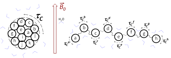
Correlation Times for Different Conformational States (folded vs. unfolded polypeptides)

Quantitatively, diffusional (“random”) molecular motions can be characterized by the correlation time \(\tau_C\), a period after which the system loses any connection to (“forgets”) its state at time zero. For example, a simplest type of random molecular motion - rotation of a spherical protein domain around its center of gravity - can be described by the correlation function \(C(t)\) which is related to the probability that the randomly moving molecule adopts its original orientation (recorded at time t=0) or conformation after a certain time \(t\). In the simplest case of an isolated folded protein, the correlation function can be expressed as

\[C(t)=C(0) e^{-t/\tau_c} \nonumber\]

where parameter \(\tau_C\) is the correlation time in this model and \(C(0)\) is the normalization factor (a number). In practical terms, the correlation time of random rotational motion of a relatively spherical folded protein (e. g., ubiquitin) can be described by the average time it takes this object to rotate by 1 radian around its center of mass (Figure \(\PageIndex{2A}\)). The probability of any subset of the target molecules returning to the original state at \(t=\tau_C\) is lower than 1 by a factor of \(1/e\), a value substantially lower than 1 (only \(1/e\) fraction of all the molecules have any chance of getting back to the original state at \(t=\tau_C\)). Thus, one can safely assume most of the target molecules “forget” their initial position or state after times equal or longer than \(\tau_C\). For folded proteins or domains, the correlation time values are relatively high (\(\tau_C > 4~\text{ns}\)) since these molecules pack tens of amino acid residues (a high-mass system) and their random rotational motion is thus quite slow. Since such molecules move and rotate roughly as a single unit, their \(\tau_C\) value is the same for all the residues in the polypeptide. For motions of amino acids in an intrinsically disordered protein (IDP) or region (IDR), each residue would move to a large degree independently from the others (a useful simplification), as if each residue behaved as a small organic molecule (Figure \(\PageIndex{3B}\)). For the residues in an IDP/IDR, their individual correlation times are small (\(\tau_C ≈ 1~\text{ns}\)), just like the values for small organic molecules. Unlike in the folded domain, an IDP would commonly need multiple correlation time values to model its internal conformational dynamics, since amino acids of various sizes can move at different rates at the same temperature (Figure \(\PageIndex{3B}\)).

Types of NMR data to probe ps-ns dynamics of biomolecules

Several types of NMR experiments produce data showing polypeptide motions in the ps-ns time range. In this chapter we will focus on \(T_1\) and \(T_2\) types of NMR data, both probing the rates (and times) of relaxation of NMR signals typically registered from the {\(\ce{^{1}H-^{15}N}\)} backbone groups in proteins. The \(T_1\) relaxation mechanism, also called spin-lattice relaxation, refers to the loss of the spin-½ excitation (and thus signal) through protein interactions with the solvent (e.g., water). Figure \(\PageIndex{3}\) (Left vs. Right) shows that the \(T_1\) relaxation times are shorter (the relaxation rates higher) for the amino acids within disordered regions (because each such residue is in direct contact with water molecules) than for the residues within folded domains where many of such residues are hidden inside the domain. The \(T_2\) relaxation mechanism, also called spin-spin relaxation, refers to the loss of the spin-½ signal coherence through internal interactions between the spins within the biomolecule itself (e.g., protein). The \(T_2\) relaxation times are typically longer (the relaxation rates lower) for the residues in IDRs, where only two neighbors (on average) are covalently bonded to each internal residue, than for residues within folded domains where each residue has many covalently and non-covalently bonded neighbors.

Figure \(\PageIndex{3}\): Left: Solvated folded protein model; Right: solvated intrinsically disordered protein (IDP); Middle: external magnetic field B0 and a graphic representing a water molecule. Note that in the IDP every residue forms a direct contact with the molecules of the solvent. Contrary to that, amino acid residues buried inside a folded protein domain are protected from interactions with water but have plenty of contact with other residues of the same protein. Finally, each “disordered” residue may have a unique correlation time value due to different sizes (masses) of the side chains. The \(\tau_C\) value for the residues in the folded domain (Left) is depicted in a larger font than for those values in the IDR to highlight the relative value difference.

The generalized free energy profile of a biomolecule (Figure \(\PageIndex{1}\)) informs us that various processes occur at drastically different time/frequency scales (Figure \(\PageIndex{2}\)). In this chapter, we focused on once class of such events - dynamics of motion of amino acids. Figures \(\PageIndex{4}\) and \(\PageIndex{4}\) combined inform us that the correlation times \(\tau_C\) for amino acid residues in folded/ordered and unfolded/disordered proteins are noticeably different (>4 ns vs. 1 ns) and that \(T_1\) and \(T_2\) rates depend on \(\tau_C\) values. Thus, \(T_1\) and \(T_2\) NMR relaxation times combined with the residue-specific NMR resonance assignment (see Chapter 6.2) can help reliably distinguish folded/ordered and unfolded/disordered elements of the protein sample. In this regard, solution NMR is one of today’s most powerful biophysical techniques. It is worth noting that in addition to \(T_1\) and \(T_2\) notation for the spin-lattice and spin-spin relaxation mechanisms, many authors use the complementary \(R1\) (\(R_1=1/T_1\)) and \(R2\) (\(R_2=1/R_2\)) notation which refers to the rates of relaxation (in units of Hz) as opposed to the relaxation times (in seconds). For a typical folded protein domain, the \(\ce{^{15}N}\) relaxation rates R1 fall into the single-digit range (in Hz) whereas the \(R2\) rates are 20-40 Hz.

Figure \(\PageIndex{4}\): Modeled \(T_1\) and \(T_2\) values (Log scale) vs correlation time \(\tau_C\) for individual residues in polymers (e.g., proteins), folded and not. Note that for small molecules or amino acids in a disordered polypeptide (\(\tau_C ≈ 1~ \text{ns}\)) the \(T_1\) and \(T_2\) values are relatively close to each other (dashed rectangle marked IDR). Contrary to that, for the residues within a typical folded domain (\(\tau_C ≥ 4~ \text{ns}\), dashed rectangle marked “Folded domains”), the \(T_2\) values are significantly shorter than \(T_1\) (>10X difference).

Big Picture

A rich repertoire of solution NMR experiments have been developed and applied in recent decades to probe biochemical and biophysical processes over time scales ranging from below picoseconds to hours and above. In addition to \(T_1\) and \(T_2\), {\(\ce{^{15}N-^{1}H}\)}-NOE (Nuclear Overhauser Effect) data provides an independent experimental probing of the ps-ns backbone motions and can distinguish between folded/ordered and unfolded/disordered domains. Another group of methods (\(R1\rho\), CPMG, CEST, etc.) produce data sensitive to motions or changes in the \(\mu \text{s-ms}\) time scale. More traditional techniques, e.g. reporting chemical shift values, can be utilized to distinguish states in slow exchange (seconds-hours). Although even a brief introduction of most of these methods is outside the scope of this text, a simple list of these approaches is enough to demonstrate that modern solution NMR is a uniquely powerful technique, capable of providing site-specific information about biomolecular structure, dynamics and function.

Further theory (optional)

A common mathematical approach relating the description of how spins involved in molecular motions and intermolecular communications at various frequencies interact with constant and alternating magnetic fields (e.g., NMR pulses) is based on the concept of the spectral density function, \(J(\omega)\). The spectral density function essentially reports a probability value J indicative of the system’s likelihood to exhibit motions or interactions happening at a given frequency \(\omega\). Mathematically, the spectral density function can be calculated as the Fourier transform of the correlation function \(C(t)\). Thus, the more complex the motions of the system, the more sophisticated its model of the correlation function needs to be and thus the more laborious it will be to propose a realistic and practically useful spectral density function. Although, \(C(t)\) and \(J(\omega)\) can be complex and even very non-trivial in many scenarios, working them out is well worth the effort as it helps to design NMR experimental schemes targeting the frequency ranges relevant for the process or sample studied. The derivation of practically used forms of \(J(\omega)\) is outside the scope of this Chapter, however at least one of the more advanced problems below provides an informative example to a curious reader.

Worked Problems

Problem \(\PageIndex{1}\)

What is the highest frequency of periodic oscillations of the smallest Newtonian objects (e.g. atoms) at room temperature and at regular body (human) temperature?

Solution

Room temperature corresponds to 25 °C (298 K), normal human body temperature is 37 °C (310 K). The oscillation frequency will be highest at \(∆G^‡ = 0\) (i.e., no barrier between the two states).

As per Equation \ref{6.3.1}, the highest frequency then is:

• at 298 K: \[\dfrac{(1.38 \times 10^{-23} ~\text{J/K}) (298~\text{K}) }{6.63 \times 10^{-34}~ \text{J} \cdot \text{s}} = 0.620 \times 10^{13}~ \text{(1/s)} \nonumber\]
• at 310 K: \[\dfrac{(1.38 \times 10^{-23} ~\text{J/K}) (310~\text{K}) }{6.63 \times 10^{-34}~ \text{J} \cdot \text{s}} = 0.645 \times 10^{13}~ \text{Hz} \nonumber\]

Problem \(\PageIndex{2}\)

What is the magnitude of the energy barrier \(∆G^‡\) between two states (A and B) of a macromolecule that corresponds to transition time of \(1~\text{ps}\) and 1 \(\mu \text{s}\) at normal human body temperature?

Solution

Transition time of \(1~\mu \text{s}\) matches to frequency \(\nu =1.00 \times 10^6~ \text{Hz} = 1~ \text{MHz}\); for 1 ps, \(\nu =1.00 \times 10^{12}~\text{Hz} = 1~ \text{THz}\).

As per Equation \ref{6.3.1}, for the transition frequency of

• \(1.00 \times 10^6~\text{Hz}\): \[\begin{align*} ∆G^‡ &= RT~ \dfrac{\ln \left(\dfrac{k_B ~ T}{h}\right)}{\nu} \\[4pt] &= 40.3 ~ \text{kJ/mol} \end{align*}\]
• \(1.00 \times 10^{12}~ \text{Hz}\): \[\begin{align*} ∆G^‡ &= RT~ \dfrac{ \ln \left( \dfrac{k_B ~ T}{h} \right)}{\nu} \\[4pt] &= 4.80 ~\text{kJ/mol} \end{align*}\]

Practice Problem \(\PageIndex{1}\)

Can the highest frequency of periodic oscillations of the smallest Newtonian objects (e.g., atoms) exceed \(10^{13}~\text{Hz}\) in a biological scenario on our planet

Practice Problem \(\PageIndex{2}\)

Chapter 3 of this text discusses molecular dynamics simulations of biological molecules. Commonly, the time step of 1 femtosecond (fs) or 2 fs are used today in these simulations to reevaluate the positions of al the atoms in the molecules and of all the forces acting upon them. The fact that these time steps are finite (non-zero) makes the simulations appear less than ideal. Given that the computational resources available today are quite extensive, would you (or would you not) suggest reducing these timesteps below 1 fs? Justify quantitatively.

Practice Problem \(\PageIndex{3}\)

As a common practice, the “\(T_1/T_2\) vs. residue number” graph for protein Q3 is provided.

(This way, less space in a journal article is used as opposed to showing two separate graphs, one for \(T_1\) and the other – for \(T_2\) as functions of the residue position in the amino acid sequence)

\(T_1/T_2\) vs. residue number” graph: The round-edge rectangles correspond to folded domains, wiggly lines to IDRs

1. How many residues does protein Q3 have?
2. Describe the 2° / 3° structure of Q3 in terms of residues belonging to folded domains vs. residues belonging to intrinsically disordered regions (IDRs).
3. What structural model, A or B, (below) corresponds to \(T_1\) and \(T_2\) NMR data for protein Q3?

Practice Problem \(\PageIndex{4}\)*

The correlation function for a spherical molecule (folded protein): \(C(t) = C(0)~ e^{-t/\tau}\). What is the algebraic expression for the spectral density function \(J(\omega)\) for this molecule? Use the obtained algebraic expression for \(J(\omega)\) to estimate the “highest rates” of rotational motion such a sample. You can define the “highest rates” as the frequency \(\omega\) value which corresponds to the \(J(\omega)\) value at 50% of its maximum.

Practice Problem \(\PageIndex{5}\)

What environmental factors and solvent properties affect the correlation time value \(\tau\) in Practice Problem \(\PageIndex{4}\) and how specifically?