6.1: 2D NMR Spectroscopy - Enhanced Spectral Resolution and Protein Backbone Conformation Reporters

This Chapter introduces 2D NMR spectroscopy, which greatly enhances the resolving power of the spectra in comparison with generic 1D data. Specifically, 2D ¹⁵N-HSQC NMR spectra will be discussed in the context of analysis of protein samples in terms of assessing chemical and conformation states of the samples. In these applications, we will be relying on the NMR basics described above: 1D NMR spectroscopy, Fourier transformation, concepts of sensitivity and resolution.

Learning Objectives

• Learn how a heteronuclear 2D NMR spectrum can greatly increase spectral resolution for large biological samples: case of ¹⁵N-HSQC
• Develop a basic sense for how ¹⁵N-labeled protein samples can be generated in the lab
• Grasp the basic information inferred for protein samples from of ¹⁵N-HSQC: peak count vs. the protein primary structure and protein states
• Learn to relate ¹⁵N-HSQC resonance positioning patterns with protein backbone conformation (folded vs. disordered) proteins
• Appreciate the role of backbone ¹H_N chemical shift values as sensitive reporters of protein backbone conformation and the role of the 8.0-8.5 ppm range

In previous sections, we introduced a very basic type of NMR data: 1D spectra, in which signal intensity depends on resonance frequency of only one type of spin-½ nuclei (e.g., ¹H). These spectra can be very informative for small molecules (MW of hundreds of Daltons) studied in organic and inorganic chemistry. In these cases, each spectrum typically has a set of well-resolved peaks whose identity in many cases can be obtained from the chemical shift values alone. The utility of such 1D NMR spectra become much more limited if they are recorded for significantly larger samples, e.g. proteins whose molecular weights often are at the level of 10 kDa and higher.

Two-dimensional (2D) NMR spectra: the case of ¹⁵N-HSQC for proteins

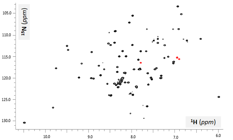
Severe spectral overlap and thus limited spectral resolution is one of the biggest limitations of 1D NMR spectra of complex biological molecules, e.g. proteins and nucleic acids. Modern NMR offers a fundamental solution to this limitation: introducing additional dimensions in the form of other types of spin-½ nuclei affecting the presence and intensity of the NMR signals. For example, let’s consider a spectrum shown in Figure VI.1.A: ¹⁵N-HSQC (Heteronuclear Single Quantum Coherence) also known as {¹H-¹⁵N}-HSQC or ¹H-¹⁵N HSQC. This is an example of a two-dimensional (2D) spectrum: the intensity of each resonance depends on two types of chemical shift values, ¹H (x-axis) and ¹⁵N (y-axis) in this case. In this type of NMR data, each spectral line corresponds to a covalent ¹⁵N-¹H group, that is a proton-nitrogen nuclear system connected by a shared electron system of a single covalent bond. This type of experiment displays significant sensitivity (high signal intensity) due to a relatively high value of proton-nitrogen scalar coupling (J-coupling) of 90-92 Hz. This value means that the the ¹H and ¹⁵N covalent partners communicate to each other changes in their magnetization states 90-92 times a second, often enough to develop a strong proton-nitrogen cross-peaks (resonance lines). No signals from protons bound to other types of atoms (carbon, oxygen, etc.) are reported. As in any type of 2D NMR data, here the signals may display significant spectral overlap in the proton (¹H) domain but since they have different ¹⁵N chemical shift values, the peaks are well-resolved. For example, for the four peaks marked with arrows their ¹H chemical shift values are very close around 8.0 ppm but they are well-resolved since their ¹⁵N shift values are all different. Thus 2D experiments offer a significant enhancement in spectral resolution in comparison with basic 1D NMR data even for large biological samples.

Figure VI.1.A ¹⁵N-HSQC of a 76-residue protein fragment. The data is courtesy of the Smirnov lab (WWU/Chemistry, Bellingham, WA).

¹⁵N-protein sample production and NH/NH2 groups contributing signals to ¹⁵N-HSQC spectra of protein samples

In order to record 15N-HSQC data, one needs to have a sufficient fraction of nitrogen atoms in the sample to be present in the from of spin-½ ¹⁵N nuclei. At their natural abundance level, 15N nuclei comprise 0.4% of all the nitrogen atoms. for protein samples, this is typically insufficient for NMR recordings since the concentration of a protein sample itself is no greater than 1 mM (typically less for most proteins). Thus methods of production of protein samples with an enhanced presence of 15N isotopes are needed. Currently, such an enrichment can be routinely achieved by expressing the target protein samples in bacterial cultures supplied with ¹⁵NH₄Cl (¹⁵N-labeled ammonium chloride) as the sole source of nitrogen for the cells. This approach allows to bring the level of uniform ¹⁵N labeling in proteins to >95%: that is >95% of all the nitrogen atoms in the sample are represented by ¹⁵N isotopes. This level is very sufficient for recording high-sensitivity ¹⁵N-HSQC data for >0.1 mM protein with the most common NMR instrumentation, e.g. at B₀ of 11.7 tesla (500 MHz of ¹H frequency) and higher. Recently, more sophisticated methods were developed, which allow for segmental labeling of large protein samples: only a portion of the protein can be labeled with NMR active isotopes to simplify the relevant NMR spectra while keeping the entire target sample present.

Almost all amino acid residues have at least one NH group present : backbone amide group. Some residues have NH and NH₂ groups within their side chains, e.g. tryptophan, asparagine, glutamine etc. One type of residues, prolines, have no NH group at all. Thus statistically for protein samples, the majority of their ¹⁵N-HSQC resonances originate from their backbone NH groups while some peaks originate from the side chains. Therefore, a simple peak count can inform the researcher about the state of the protein sample by answering a simple question: does the ¹⁵N-HSQC peak count correspond (or not) to the primary structure of the sample? [Let’s recall that a protein primary structure is defined as its amino acid sequence plus all the relevant post-translational covalent modifications like phosphorylation, disulfide bonds, ubiquitination, methylation, etc.]. If the number of the resonances (“cross-peaks”) is equal to the number of signals expected from the protein primary structure than one can propose that the sample has a single conformation (and chemical) state. If the number of the observed ¹⁵N-HQC peaks is greater than what is predicted from the protein’s primary structure then one can conclude that the protein exists in multiple conformational and/or chemical states. If the number of observed peaks is too small for the sample of a certain primary structure, some more complex scenarios need to be expected: aggregation, complex dynamics behavior, chemical degradation etc. These scenarios will be discussed later in this and other chapters of this part of the textbook. Table IV.1.I sums up these scenarios.

Table IV.1.I

The number of ^15N-HSQC resonances: observed vs. expected	Most likely protein sample state
Observed ≈ Expected	Single average conformation and single chemical state (no degradation)
Observed >> Expected	Multiple conformational states or chemical degradation possible
Observed << Expected	Possible aggregation and/or complex dynamics regimes

¹⁵N-HSQC and conformation states of protein backbone: folded/ordered vs. unfolded/disordered samples

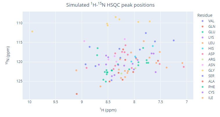
In addition to the analysis of the number of ¹⁵N-HSQC resonances, the way the signals are positioned within the spectrum (peak pattern) is very informative as well. Since most of the ¹⁵N-HSQC peaks originate from the backbone amides, ¹H chemical shift values can be used to assess the chemical/electronic environment for the residues and thus can work as reliable reporters of the backbone state: folded vs. unfolded. The ¹⁵N-HSQC spectrum in Figure VI.1.A corresponds to a mostly folded polypeptide as can be judged by the fact that most of the resonances have ¹H_N chemical shift values are found outside of 8.0-8.5 ppm window. This significant dispersion of the peaks in the amide proton dimension indicates that for most of residues, their electronic environment of their backbone amide groups is unique for each residues, which can only be the case for a folded protein (each backbone HN group has different set of non-covalent neighbors). Contrary to that, a disordered polypeptide exposes its backbone HN groups to nearly identical environments, which is mostly water. Therefore, the ¹⁵N-HSQC resonances of an intrinsically disordered protein (IDP) or an intrinsically disordered region (IDR) will be clustered within a narrow range of 1HN chemical shift values, typically within 8.0-8.5 ppm as shown on Figure VI.1.B.

Figure VI.1.B A schematic ¹⁵N-HSQC spectrum of an intrinsically disordered protein (IDP). Note that most of the signals are clustered within 8.0-8.5 ppm in ¹H dimension.

Examples

Example \(\PageIndex{1}\)

A high number of chemical shift data is currently available for all the 20 amino acids in isolation or for their respective ¹H and ¹⁵N resonances in the context of protein samples. Biological Magnetic Resonance Data Bank (BMRB) provides public access to this information with very useful statistics:

Using the BMRB chemical shift statistics, rank the average backbone ¹⁵NH chemical shift values for the following types of amino acids: Ala, Gly, Trp.

Answer

BMRB chemical shift table gives the following average ¹⁵NH values and rank for the three residue types:

Gly (109.6 ppm) < Trp (121.6 ppm) < Ala (123.3 ppm)

As we can see, Gly backbone nitrogen chemical shifts are noticeably lower than for the other two residue types. In fact, Gly is similarly different from all other residue types as well.

Example \(\PageIndex{2}\)

How many residues can be estimated to belong to ordered (folded) segments of protein sample for BMRB Entry 50205?

Answer

Examination of the ¹⁵N-HSQC of BMRB entry 50205 reveals about 75-85 signals outside of 8.0-8.5 ppm ¹H_N chemical shift range.

Some peaks corresponding to Asn and Gln side chains need to be excluded from the cumulative statistics (see Practice Problem 2 below).

Practice Problems

Problem 1. List all the standard amino acids whose side chains have NH or NH₂ groups. List all the standard amino acids which have no NH, NH₂ and NH₃⁺ groups when place internally within a polypeptide chain.

Problem 2. Predict an ¹⁵N-HSQC peak pattern and their approximate location on the spectrum (use Figure VI.1.B as template) for side chains of Asn and Gln residues.

Problem 3. Predict an ¹⁵N-HSQC peak pattern and their approximate location on the spectrum (use Figure VI.1.B as template) for side chains of Trp residues.

Problem 4. Why are backbone ¹H_N chemical shift values are more reliable indicators or folded vs. disordered backbone states of a protein than backbone ¹⁵N_H values? Thinking simplistically, both nuclei form covalent backbone amide groups and thus can be equally sensitive reporters of the protein backbone conformations. However, we see that the ¹⁵N_H chemical shift values do not change much upon unfolding or folding of a polypeptide whereas ¹H_N ones undergo major and easily detectible changes as Figures VI.1A and VI.1.B above show. Explain.

Problem 5. Estimate (with a justification) how many residues may belong to disordered segments of the backbone for protein sample delivering the ¹⁵N-HSQC spectrum shown in Figure VI.1.A.

Problem 6*. Estimate (with a justification) how many residues may belong to ordered (folded) segments of the backbone for protein sample delivering the ¹⁵N-HSQC spectrum shown in Figure VI.1.B.

Problem 7*. Example 2 above indicates that protein sample for BMRB entry 50205 likely has 75-85 “folded” residues. How many residues can be estimated to belong to disordered (unfolded) segments in this 183-redsidue protein sample?