7.2: Background

Background

Indicator Titrations

The next several labs will involve laboratory techniques that take into account the equilibrium chemistry associated with the stoichiometry of chemical reactions. The first will involve titrations of acid base reactions that may include the equilibria of weak acids or bases and the second will deal with the formation of complex ions.  The stoichiometry of acid base titrations were introduced in the first semester (section 4.7) as an analytical technique to determine the concentration of an unknown (analyte) by adding a standard of known concentration (titrant) until they were in stoichiometric proportions (the equivalence point).  At the equivalence point the analyte has been neutralized and converted to its salt (conjugate form). The volume of titrant required to neutralize the analyte could be quickly determined through the use of an appropriate indicator, where titrant was added until the solution changed color, which was at a volume known as the endpoint of the titration.  For this to work the pH at which an indicator changes color must be the same as that of the salt of the analyte being neutralized. The analyte may be weak or strong, but the titrant must be strong and typically is monoprotic. Figure  \(\PageIndex{2}\) shows the experimental setup for an indicator based titration

Figure \(\PageIndex{2}\): Setup for using an indicator to determine the concentration of an unknown through a titration. 

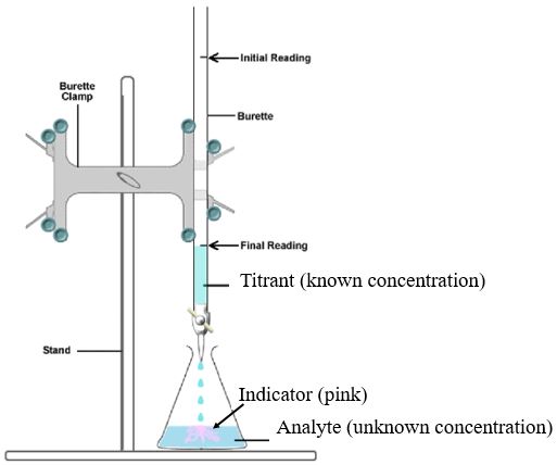
Figure \(\PageIndex{6}\) of the experimental section is a chart of the colors and pHs various indicators change at and it is important that you pick an appropriate indicator based on the acidity or basicity of the neutralized analyte.  If the analyte is a strong acid or base the indicator should change color around a pH of 7.  If the analyte is a weak acid the indicator should change color in a basic solution, and if it is a weak base it should change color in an acidic solution.  The calculations for determining this are in the expermintal section of this lab.

pH Titrations

In a pH titration you measure the pH as a function of the volume of titrant added and determine the equivalence point as the point in where there is an inflection in the slope of the curve.  Figure \(\PageIndex{2}\) shows the four common types of titrations.  Initially the pH is that of the pure analyte. Before the equivalence point the titrant is neutralizing the analyte and converting it to its salt, but since there is an excess of the analyte it is not completely consumed and so a buffer is formed, which is a mixture of the analyte and its salt. As the equivalence point is approached the pH changes rapidly as the analyte is being consumed and so there is nothing to react with the titrant (which must be a strong acid or base) and after the equivalence point the pH stabilizes as it is effectively determined by the pure titrant, which is both strong and in excess, and a change is only due to dilution.  Lets look at two examples

1. Titration of Acetic Acid with Sodium hydroxide (analagous to figure \(\PageIndex{3}\)c.  Initially the pH is due to pure acetic acid . As sodium hydroxide is added it reacts with the acetic acid forming its conjugate base,  the salt sodium acetate.  This is an acetic acid/acetate buffer and the pH is determined by the ratio of the un-neutralized to neutralized acetic acid.
   \[C_2H_3O_2(aq) + NaOH(aq)  \rightarrow NaC_2H_3O_2(aq) + H_2O(l) \]
   At the equivalence point all the acetic acid  has been neutralized  and converted to its conjugate base acetate, so the pH is determined by the concentration of its salt, sodium acetate.  After the equivalence point there is no more acetic acid to react with the sodium hydroxide and so it accumulates, with the pH being dictated by the amount of excess sodium hydroxide.
2. Titration of Ammonia with Hydrochloric Acid (analagous to figure \(\PageIndex{3}\)d.  Initially the pH is due to pure ammonia  As HCl is added it reacts with the ammonia forming its salt, ammonium chloride.  This is an ammonia/ammonium buffer and the pH is determined by the ratio of the un-neutralized to neutralized ammonia.
   \[NH_3(aq) + HCl(aq) \rightarrow NH_4Cl(aq)  \]
   At the equivalence point  all the ammonia has been neutralized and converted to its conjugate acid ammonium, and so the pH is dictated by the concentration of the ammonium chloride salt.  After the equivalence point there is no more ammonia to react with the HCl and so it accumulates and the pH is dictated by the excess HCl.

 

 

Figure \(\PageIndex{3}\): Titration curves for (a) strong acid with strong base and (b) strong base with strong acid.

Equivalence Point Determination

A closer look at figure \(\PageIndex{3}\) indicates that the steepest part of the titration curve is the equivalence point and that there is an inflection in the slope of the line as the solution goes from excess analyte to excess titrant.  Lets look at parts (a) and (c) of figure \(\PageIndex{3}\).  As you approach the equivalence point the slope increases and then after the equivalence it decreases.  This can be shown with a first derivative plot of the curve as in figure \(\PageIndex{4}\) \(\left ( lim \;\Delta V \to 0 \;  \frac{\Delta pH}{\Delta V} \right )\) .  What is clear in the first derivative plot is that the line is going higher and higher and then reverses direction and goes lower and lower.  The point where it changes from increasing to decreasing is the inflection point, and this can identified where the second derivative plot goes through zero \(\left ( lim \;\Delta V \to 0 \;  \frac{\Delta^2 pH}{\Delta V^2} \right )\) . Note, if there is noise in your data over the flat portion of the curve you will have a lot of false inflection points and so you do not need to take the second derivitive plot over all the data, just in the region around the equivalence point

 

Figure \(\PageIndex{4}\): pH Tiration curve with first and second derivative plots. (Belford cc 0)

 

Titration of a weak monoprotic acid.

Figure \(\PageIndex{4}\) shows the four "regions" of the titration curve for the titration of a weak acid with a strong base. It should be noted that region two is a buffer because there is excess acid (analyte) and so only part of it been neutralized by the base and converted to it's salt (the acid's conjugate base). This is one of the two ways to make a buffer (see section 17.2.3).

Weak Acid + Strong Base -> Salt +Water

where the salt is the conjugate base of the acid.

The four parts of the titration curve are described below and you should look to the approriate text section to see how they are treated.

1. Pure Acid (0 ml of base is added, section 17.3.2.1)
2. Excess acid (you have not added enough base to neutralize all of it and so have a buffer of the weak acid and it's salt, section 17.3.2.2)
   • K_a can be calculated from the pH at half equivalence (section 17.3.2.2.1)
3. Equivalence Point (the acid and base are in stoichiometric proportions and you effectively have the salt of the weak acid, section 17.3.2.3)
   • The acid and base are in 1 to 1 ratio at the equivalence point and so the initial moles acid can be calculated from the moles base at this point (n_A=n_B and n_B=M_BV_B)
     • If the acid was a solution you can determine its molarity from he volume titrated.
     • If the acid was a solid you can determine its molar mass from the mass titrated.
4. Excess Base (you have added more base than there was acid, section 17.3.2.4)

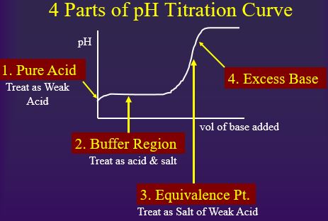
Figure  \(\PageIndex{5}\): Four parts of the titration curve for a weak acid being titrated with a strong base. Notice that two parts are points (1 & 3) and two parts are regions (2 & 4).

Be sure to go over the four parts of the titration curve in section 17.3.2 as that material is not being repeated here.  If you are titrating a weak base with a strong acid you should go over section 17.3.4

 

Titration of Weak Diprotic Acid

A diprotic acid has two titratable protons and if K_a1>1000K_a2 there are two clearly defined equivalence points.

Determination of K_a

K_a can be determined by reading the pH at half equivalence (when half of the acid has been neutralized and converted to its salt).  This is in the buffer region and uses the Henderson Hasselbach equation

\[pH=pK_a+\log \dfrac{[A^-]}{HA}\]

Since at half equivalence [HA]=[A^-] pH = pK_a , at half equivalence

so 

\[K_a =10^{-pH\text{, at half equivalence}} \]

So you find the equivalent point on the titration curve and read the value of the curve at half of that volume.  For this reason you need to collect data half way along the curve (red circle).

pH Probes

In this experiment we will use a Ph probe, which is an electronic device that measures the pH. These are very common and they should always be checked against standard solutions of known pH and calibrated if they read incorrectly. The pH probe is an electrochemical cell and we will cover these in chapter 19, sections 19.3-19.5 and 19.7. The following YouTube from Oxford Press does an excellent job of describing how a pH probe works.  It is imperative that you test your probe in a buffer to be sure it is reading accurately and if it is not, you will need to calibrate it.

Video \(\PageIndex{1}\) 2:30 YouTuve describing the operation of a pH probe developed by Oxford University Press (https://youtu.be/aIn4D2QXUy4).

The pH reading is not accurate until the probe stabilizes, so when you change the pH you need to wait until the reading becomes steady before recording the value.

Exploratory Run

Before running a pH titration you should make a trial run with an indicator (section 17.3.4.2), which is a chemical that undergoes a color change at a specific pH.  You want an indicator that indicates when the titrant and analyte have been added in stoichiometric proportions, (the equivalence point), which is when the analyte has been converted to its salt. From section 17.3.3.2 we see that for the titration of a weak acid

\[[OH^-]=\sqrt{\left (\frac{K_w}{K_a} \right )[A^-]_e} \]

where K_w=water ionization constant (10^-14), K_a=acid ionization constant and [A^-_e]=the salt concentration at the equivalence point (when all the acid is neutralized). 

So  \[pOH =-log\sqrt{\left (\frac{K_w}{K_a} \right )[A^-]_e} \]

and \[pH=14-pOH=14+ \sqrt{\left (\frac{K_w}{K_a} \right )[A^-]_e} \]

In the first experiment we are neutralizing 25.00 mL of 0.100M acetic acid with 0.100M NaOH, and so when 25.00 mL of NaOH has been added all the acetic acid will be converted to acetate ions, but the volume has doubled and so the concentration is now 0.05M A^-.  This gives a pH of 

\[pH=14-pOH=14+ \sqrt{\left (\frac{10^{-14}}{1.8x10^{-5}} \right )[0.05M]_e}= 8.72\]

From figure \(\PageIndex{4}\) we see that phenolphthalein would be a good indicator for a weak acid like acetic acid as it is clear up until just below a pH of 9, when it turns pink.

Figure \(\PageIndex{6}\): Common indicators and pH ranges they change color

 

That is, you want an indicator that changes color at the pH of the salt of the acid or base that you are titrating, and that way you can tell when you have completely neutralized it.