
7.3: Procedures
- Page ID
- 379602
\( \newcommand{\vecs}[1]{\overset { \scriptstyle \rightharpoonup} {\mathbf{#1}} } \)
\( \newcommand{\vecd}[1]{\overset{-\!-\!\rightharpoonup}{\vphantom{a}\smash {#1}}} \)
\( \newcommand{\id}{\mathrm{id}}\) \( \newcommand{\Span}{\mathrm{span}}\)
( \newcommand{\kernel}{\mathrm{null}\,}\) \( \newcommand{\range}{\mathrm{range}\,}\)
\( \newcommand{\RealPart}{\mathrm{Re}}\) \( \newcommand{\ImaginaryPart}{\mathrm{Im}}\)
\( \newcommand{\Argument}{\mathrm{Arg}}\) \( \newcommand{\norm}[1]{\| #1 \|}\)
\( \newcommand{\inner}[2]{\langle #1, #2 \rangle}\)
\( \newcommand{\Span}{\mathrm{span}}\)
\( \newcommand{\id}{\mathrm{id}}\)
\( \newcommand{\Span}{\mathrm{span}}\)
\( \newcommand{\kernel}{\mathrm{null}\,}\)
\( \newcommand{\range}{\mathrm{range}\,}\)
\( \newcommand{\RealPart}{\mathrm{Re}}\)
\( \newcommand{\ImaginaryPart}{\mathrm{Im}}\)
\( \newcommand{\Argument}{\mathrm{Arg}}\)
\( \newcommand{\norm}[1]{\| #1 \|}\)
\( \newcommand{\inner}[2]{\langle #1, #2 \rangle}\)
\( \newcommand{\Span}{\mathrm{span}}\) \( \newcommand{\AA}{\unicode[.8,0]{x212B}}\)
\( \newcommand{\vectorA}[1]{\vec{#1}} % arrow\)
\( \newcommand{\vectorAt}[1]{\vec{\text{#1}}} % arrow\)
\( \newcommand{\vectorB}[1]{\overset { \scriptstyle \rightharpoonup} {\mathbf{#1}} } \)
\( \newcommand{\vectorC}[1]{\textbf{#1}} \)
\( \newcommand{\vectorD}[1]{\overrightarrow{#1}} \)
\( \newcommand{\vectorDt}[1]{\overrightarrow{\text{#1}}} \)
\( \newcommand{\vectE}[1]{\overset{-\!-\!\rightharpoonup}{\vphantom{a}\smash{\mathbf {#1}}}} \)
\( \newcommand{\vecs}[1]{\overset { \scriptstyle \rightharpoonup} {\mathbf{#1}} } \)
\( \newcommand{\vecd}[1]{\overset{-\!-\!\rightharpoonup}{\vphantom{a}\smash {#1}}} \)
\(\newcommand{\avec}{\mathbf a}\) \(\newcommand{\bvec}{\mathbf b}\) \(\newcommand{\cvec}{\mathbf c}\) \(\newcommand{\dvec}{\mathbf d}\) \(\newcommand{\dtil}{\widetilde{\mathbf d}}\) \(\newcommand{\evec}{\mathbf e}\) \(\newcommand{\fvec}{\mathbf f}\) \(\newcommand{\nvec}{\mathbf n}\) \(\newcommand{\pvec}{\mathbf p}\) \(\newcommand{\qvec}{\mathbf q}\) \(\newcommand{\svec}{\mathbf s}\) \(\newcommand{\tvec}{\mathbf t}\) \(\newcommand{\uvec}{\mathbf u}\) \(\newcommand{\vvec}{\mathbf v}\) \(\newcommand{\wvec}{\mathbf w}\) \(\newcommand{\xvec}{\mathbf x}\) \(\newcommand{\yvec}{\mathbf y}\) \(\newcommand{\zvec}{\mathbf z}\) \(\newcommand{\rvec}{\mathbf r}\) \(\newcommand{\mvec}{\mathbf m}\) \(\newcommand{\zerovec}{\mathbf 0}\) \(\newcommand{\onevec}{\mathbf 1}\) \(\newcommand{\real}{\mathbb R}\) \(\newcommand{\twovec}[2]{\left[\begin{array}{r}#1 \\ #2 \end{array}\right]}\) \(\newcommand{\ctwovec}[2]{\left[\begin{array}{c}#1 \\ #2 \end{array}\right]}\) \(\newcommand{\threevec}[3]{\left[\begin{array}{r}#1 \\ #2 \\ #3 \end{array}\right]}\) \(\newcommand{\cthreevec}[3]{\left[\begin{array}{c}#1 \\ #2 \\ #3 \end{array}\right]}\) \(\newcommand{\fourvec}[4]{\left[\begin{array}{r}#1 \\ #2 \\ #3 \\ #4 \end{array}\right]}\) \(\newcommand{\cfourvec}[4]{\left[\begin{array}{c}#1 \\ #2 \\ #3 \\ #4 \end{array}\right]}\) \(\newcommand{\fivevec}[5]{\left[\begin{array}{r}#1 \\ #2 \\ #3 \\ #4 \\ #5 \\ \end{array}\right]}\) \(\newcommand{\cfivevec}[5]{\left[\begin{array}{c}#1 \\ #2 \\ #3 \\ #4 \\ #5 \\ \end{array}\right]}\) \(\newcommand{\mattwo}[4]{\left[\begin{array}{rr}#1 \amp #2 \\ #3 \amp #4 \\ \end{array}\right]}\) \(\newcommand{\laspan}[1]{\text{Span}\{#1\}}\) \(\newcommand{\bcal}{\cal B}\) \(\newcommand{\ccal}{\cal C}\) \(\newcommand{\scal}{\cal S}\) \(\newcommand{\wcal}{\cal W}\) \(\newcommand{\ecal}{\cal E}\) \(\newcommand{\coords}[2]{\left\{#1\right\}_{#2}}\) \(\newcommand{\gray}[1]{\color{gray}{#1}}\) \(\newcommand{\lgray}[1]{\color{lightgray}{#1}}\) \(\newcommand{\rank}{\operatorname{rank}}\) \(\newcommand{\row}{\text{Row}}\) \(\newcommand{\col}{\text{Col}}\) \(\renewcommand{\row}{\text{Row}}\) \(\newcommand{\nul}{\text{Nul}}\) \(\newcommand{\var}{\text{Var}}\) \(\newcommand{\corr}{\text{corr}}\) \(\newcommand{\len}[1]{\left|#1\right|}\) \(\newcommand{\bbar}{\overline{\bvec}}\) \(\newcommand{\bhat}{\widehat{\bvec}}\) \(\newcommand{\bperp}{\bvec^\perp}\) \(\newcommand{\xhat}{\widehat{\xvec}}\) \(\newcommand{\vhat}{\widehat{\vvec}}\) \(\newcommand{\uhat}{\widehat{\uvec}}\) \(\newcommand{\what}{\widehat{\wvec}}\) \(\newcommand{\Sighat}{\widehat{\Sigma}}\) \(\newcommand{\lt}{<}\) \(\newcommand{\gt}{>}\) \(\newcommand{\amp}{&}\) \(\definecolor{fillinmathshade}{gray}{0.9}\)Experimental Procedures
Before running a pH titration we are going to make a quick exploratory run with an indicator. The endpoint of an indicator titration is when the indicator changes color and if we choose an indicator that changes color at the pH of the salt of the analyte, it gives us a bearing on the equivalence point, which is when that analyte and titrant have been added in stoichiometric proportions (moles acid = moles base for monoprotic acid being titrated with a monoprotic base). You will then use the results of the exploratory run to design the pH titration.
Designing the pH titration
The challenge is that the pH probes are old and it takes a while for their readings to stabilize. If you do not let the reading stabilize there will be a lot of noise in your data.
 Figure \(\PageIndex{7}\): Dots represent pH readings. (Copyright; Belford CC-BY)
The goal of the exploratory run is to figure out where the equivalence point is. You then need to record data dropwise for about 3/4 a mL before and after the endpoint and collect data around half equivalence. You need to be sure to record the inital pH (pure acid) and extend your data at least 5 mL beyond the equivalence point.
Tips on getting good data
If you look at YouTube you will see many titrations where people are creating a vortex with magnetic stirrers. This can increase the rate at which gasses dissolve and there are a class of non-metal oxides called the acid anhydrides that form acids when they combine with water. The carbon dioxide you exhale is an acid anhydride and the following youtube shows what happens if you breath over a beaker that is rapidly being stirred.
Video \(\PageIndex{2}\): 1:10 minute video showing effect of cavitation and breathing on a slightly basic solution (https://youtu.be/4RiftqpXI8c, Belford)
In the above video a slightly basic solution with phenolphthalein indicator is pink. If you listen carefully you can hear someone breathing above it and due to the vortex the carbon dioxide they exhale reacts with the water to form carbonic acid and the solution turns clear.
\[CO_2(g) +H_2O(l) \leftrightharpoons H_2CO_3(aq)\]
Exploratory Run
The goal of the exploratory run is to give you a feeling for the volume of actual titrant you will need to neutralize 25 mL of your analyte. Using a volumetric pipette 25 mL of acetic acid and a few drops of phenolphthalein were added to the Erlenmeyer flask. Then it was titrated with 0.1M NaOH and the volume of NaOH needed to neutralize the acetic acid was quickly determined. This video shows how to quickly do this, and we are not using this to measure the concentration, but to get a quick bearing on how to design the pH titration.
Video \(\PageIndex{3}\): 2:01 minute video showing a quick exploratory run with an indicator. Note how as the titration proceeds the color takes longer to disappear as the solution approaches the end point.
pH Run
In this experiment we will hook up the Vernier pH probe to a $35 Raspberry Pi microcomputer that transmits the data to your Google Sheet in real time. We will run two python programs on the Raspberry Pi. The first program we will run from the command line and it gives you the pH readings every 10 seconds, and you use this to decide when to upload data to your Google Sheet. The second program you will run from the Thonny IDE (Interactive Development Environment), and this program will allow you to input your volumes and pH to your Google Sheet. These programs were developed during the COVID pandemic to allow instructors to stream data to students in real time, and we have decided to let students use them directly, as data science skills are important for today's students to learn. Further information may be obtained in the Internet of Science Things course at UALR. Please do not get water on the Raspberry Pis as you will kill them.
 Figure \(\PageIndex{8}\): Raspberry Pi in "Desktop mode" hooked up to a pH probe. Note, this Pi is also hooked up to a breadboard (Copyright; Bob Belford, CC-BY)
COVID 19 Protocols
The second reason we have decided to use the Raspberry Pis is that we feel the lab can be run safer in a pandemic than using the normal equipment. We ask students to take up roles for each experiment, and change the roles when they perform different titrations. Note, at the discretion of your instructor these roles may be modified by the number of people in your group. Each group will have two stations on opposite sides of the bench. On one side is the Raspberry Pi, keyboard and monitor, and on the other side is the titration setup. All students need to work together, make sure the lab is run safely and that you get the best data possible.
- Titrator. Only one person handles the buret (opens and closes the stopcock).
- burette reader. This person assists the titrator and reads the volume. This may be the person running the titration.
- Titration supervisor. This person coordinates with the titrator and burette reader to determine the approriate volumes for when they should make a measurement and for communicating with the data supervisor.
- Pi operator. This is the only person who touches the keyboard and mouse. This person runs the python programs.
- Data supervisor. This person assists the pi operator in determining when the pH is stable enough to upload to the Google Sheet, and is responsible for communicating with the titration supervisor.
IOT Enhanced Titration
The following image shows the setup for the titration lab. Note this Raspberry Pi is being run in "headless mode" through VNC viewer and connected to a laptop. Your Pi may be run in desktop mode, where it is connected to a monitor and keyboard. Note the tip of the pH probe is submerged and magnetic stirrer is set where it is under the burette and does not touch the probe as it spins. A gentle spin is all you need.
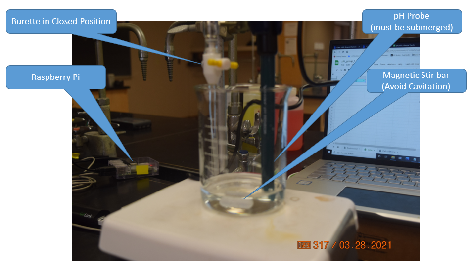
Be sure to add enough water to submerge the pH probe and take the dilution effect of this water into account when determining the initial concentration of the acid.
The following image shows all the programs on the desktop of a Raspberry Pi (remotely accessed via VNC viewer). Step (1) of the blue commands show you how to run the "current pH" program in command line, where (2) shows the display with the values being streamed every 10 seconds. The green tabs show how to activate and run the progam that sends data to the Google Sheet (ph_Venier_sheets.py). (1) Open the folder pH_lab on the desktop and then (2) clicking the python program pH_Veneir_sheets.py opens that program in the Thonny. The shell of Thonny (3) allows you to input the volume in mL (do not include units) and when you hit <enter> that volume and the current pH are uploaded to the Google Sheet. You need to use both progams concurrently.
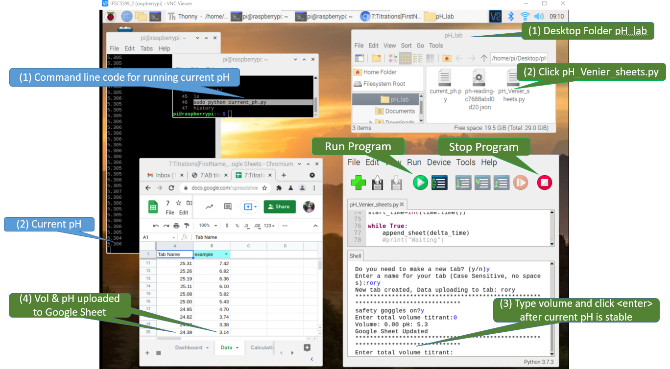 Figure \(\PageIndex{10}\): The Raspberry Pi Desktop is being overlaid a Google sheet by the VNC Vierwer in this screen capture. There are two Python programs being run, one in command line and one in the Thonny IDE (Interactive Development Environment). The white text on the black background is the program being run in command line and every 10 seconds it displays the current pH. The program in Thonny is running a program "PH_Vernier_sheets_append", which allows a user to enter the volume and when the hit <Enter> it takes that volume and pH and appends it to the Google Sheet in the foreground. (Bob Belford, CC-BY)
Stepwise procedures
- Add titrant
- Record the new volume of titrant added to analyte in Thonny Shell (running pH_Venier_sheets.py)
- Observe pH in command line (running current_pH.py)
- When pH is stable, hit <enter> on Thonny
- repeat above steps with a new volume of titrant
Note, you do not need to run the Google Sheet, but it would be nice to be sure your data is being uploaded (everytime you hit enter on Thonny your sheet should be updated). You can also run the Google Sheet on a separate laptop.
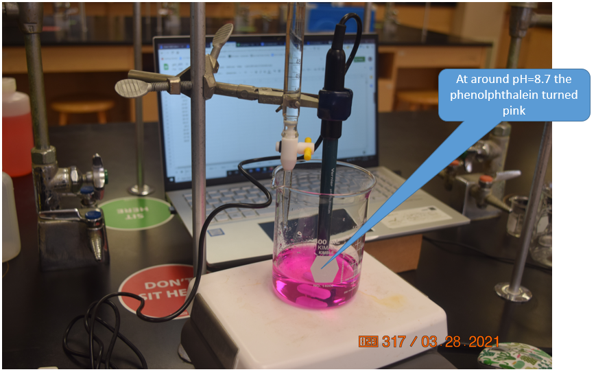 Figure \(\PageIndex{11}\): At around pH=8.7 the indicator turned pink, and the titration was continued for another 5 mL into the excess base region. As there was only one person in the lab we ignored the COVID-19 seating assignments, but if students attend labs they need to sit where the green stickers are (Belford, cc 3.0)
Printable Instructions