
7.4: Data Analysis
- Page ID
- 379603
\( \newcommand{\vecs}[1]{\overset { \scriptstyle \rightharpoonup} {\mathbf{#1}} } \)
\( \newcommand{\vecd}[1]{\overset{-\!-\!\rightharpoonup}{\vphantom{a}\smash {#1}}} \)
\( \newcommand{\id}{\mathrm{id}}\) \( \newcommand{\Span}{\mathrm{span}}\)
( \newcommand{\kernel}{\mathrm{null}\,}\) \( \newcommand{\range}{\mathrm{range}\,}\)
\( \newcommand{\RealPart}{\mathrm{Re}}\) \( \newcommand{\ImaginaryPart}{\mathrm{Im}}\)
\( \newcommand{\Argument}{\mathrm{Arg}}\) \( \newcommand{\norm}[1]{\| #1 \|}\)
\( \newcommand{\inner}[2]{\langle #1, #2 \rangle}\)
\( \newcommand{\Span}{\mathrm{span}}\)
\( \newcommand{\id}{\mathrm{id}}\)
\( \newcommand{\Span}{\mathrm{span}}\)
\( \newcommand{\kernel}{\mathrm{null}\,}\)
\( \newcommand{\range}{\mathrm{range}\,}\)
\( \newcommand{\RealPart}{\mathrm{Re}}\)
\( \newcommand{\ImaginaryPart}{\mathrm{Im}}\)
\( \newcommand{\Argument}{\mathrm{Arg}}\)
\( \newcommand{\norm}[1]{\| #1 \|}\)
\( \newcommand{\inner}[2]{\langle #1, #2 \rangle}\)
\( \newcommand{\Span}{\mathrm{span}}\) \( \newcommand{\AA}{\unicode[.8,0]{x212B}}\)
\( \newcommand{\vectorA}[1]{\vec{#1}} % arrow\)
\( \newcommand{\vectorAt}[1]{\vec{\text{#1}}} % arrow\)
\( \newcommand{\vectorB}[1]{\overset { \scriptstyle \rightharpoonup} {\mathbf{#1}} } \)
\( \newcommand{\vectorC}[1]{\textbf{#1}} \)
\( \newcommand{\vectorD}[1]{\overrightarrow{#1}} \)
\( \newcommand{\vectorDt}[1]{\overrightarrow{\text{#1}}} \)
\( \newcommand{\vectE}[1]{\overset{-\!-\!\rightharpoonup}{\vphantom{a}\smash{\mathbf {#1}}}} \)
\( \newcommand{\vecs}[1]{\overset { \scriptstyle \rightharpoonup} {\mathbf{#1}} } \)
\( \newcommand{\vecd}[1]{\overset{-\!-\!\rightharpoonup}{\vphantom{a}\smash {#1}}} \)
\(\newcommand{\avec}{\mathbf a}\) \(\newcommand{\bvec}{\mathbf b}\) \(\newcommand{\cvec}{\mathbf c}\) \(\newcommand{\dvec}{\mathbf d}\) \(\newcommand{\dtil}{\widetilde{\mathbf d}}\) \(\newcommand{\evec}{\mathbf e}\) \(\newcommand{\fvec}{\mathbf f}\) \(\newcommand{\nvec}{\mathbf n}\) \(\newcommand{\pvec}{\mathbf p}\) \(\newcommand{\qvec}{\mathbf q}\) \(\newcommand{\svec}{\mathbf s}\) \(\newcommand{\tvec}{\mathbf t}\) \(\newcommand{\uvec}{\mathbf u}\) \(\newcommand{\vvec}{\mathbf v}\) \(\newcommand{\wvec}{\mathbf w}\) \(\newcommand{\xvec}{\mathbf x}\) \(\newcommand{\yvec}{\mathbf y}\) \(\newcommand{\zvec}{\mathbf z}\) \(\newcommand{\rvec}{\mathbf r}\) \(\newcommand{\mvec}{\mathbf m}\) \(\newcommand{\zerovec}{\mathbf 0}\) \(\newcommand{\onevec}{\mathbf 1}\) \(\newcommand{\real}{\mathbb R}\) \(\newcommand{\twovec}[2]{\left[\begin{array}{r}#1 \\ #2 \end{array}\right]}\) \(\newcommand{\ctwovec}[2]{\left[\begin{array}{c}#1 \\ #2 \end{array}\right]}\) \(\newcommand{\threevec}[3]{\left[\begin{array}{r}#1 \\ #2 \\ #3 \end{array}\right]}\) \(\newcommand{\cthreevec}[3]{\left[\begin{array}{c}#1 \\ #2 \\ #3 \end{array}\right]}\) \(\newcommand{\fourvec}[4]{\left[\begin{array}{r}#1 \\ #2 \\ #3 \\ #4 \end{array}\right]}\) \(\newcommand{\cfourvec}[4]{\left[\begin{array}{c}#1 \\ #2 \\ #3 \\ #4 \end{array}\right]}\) \(\newcommand{\fivevec}[5]{\left[\begin{array}{r}#1 \\ #2 \\ #3 \\ #4 \\ #5 \\ \end{array}\right]}\) \(\newcommand{\cfivevec}[5]{\left[\begin{array}{c}#1 \\ #2 \\ #3 \\ #4 \\ #5 \\ \end{array}\right]}\) \(\newcommand{\mattwo}[4]{\left[\begin{array}{rr}#1 \amp #2 \\ #3 \amp #4 \\ \end{array}\right]}\) \(\newcommand{\laspan}[1]{\text{Span}\{#1\}}\) \(\newcommand{\bcal}{\cal B}\) \(\newcommand{\ccal}{\cal C}\) \(\newcommand{\scal}{\cal S}\) \(\newcommand{\wcal}{\cal W}\) \(\newcommand{\ecal}{\cal E}\) \(\newcommand{\coords}[2]{\left\{#1\right\}_{#2}}\) \(\newcommand{\gray}[1]{\color{gray}{#1}}\) \(\newcommand{\lgray}[1]{\color{lightgray}{#1}}\) \(\newcommand{\rank}{\operatorname{rank}}\) \(\newcommand{\row}{\text{Row}}\) \(\newcommand{\col}{\text{Col}}\) \(\renewcommand{\row}{\text{Row}}\) \(\newcommand{\nul}{\text{Nul}}\) \(\newcommand{\var}{\text{Var}}\) \(\newcommand{\corr}{\text{corr}}\) \(\newcommand{\len}[1]{\left|#1\right|}\) \(\newcommand{\bbar}{\overline{\bvec}}\) \(\newcommand{\bhat}{\widehat{\bvec}}\) \(\newcommand{\bperp}{\bvec^\perp}\) \(\newcommand{\xhat}{\widehat{\xvec}}\) \(\newcommand{\vhat}{\widehat{\vvec}}\) \(\newcommand{\uhat}{\widehat{\uvec}}\) \(\newcommand{\what}{\widehat{\wvec}}\) \(\newcommand{\Sighat}{\widehat{\Sigma}}\) \(\newcommand{\lt}{<}\) \(\newcommand{\gt}{>}\) \(\newcommand{\amp}{&}\) \(\definecolor{fillinmathshade}{gray}{0.9}\)Data Analysis
Accessing your Data
The program on the raspberry pi automatically sends the data to your instructor, which is then sent to your copy of the workbook template. Make your copy of the template from the 7.3 Titrations Lab Report and rename the title to be your name.
Navigate to the data tab and click the drop down in cell B1 to find your group. (The name you chose when starting the program) Next click the #REF in cell A2 and select Allow access. Now you should automatically see your groups data.
If you do not see your group's name ask the instructor to refresh the Index
Highlight the cells you want to copy then go to the tab you want to use. You want to paste values only so you can use Ctrl+Shift+V or right click and select Paste Values Only.
Week 1
Titration Curve
First make your titration curve (First image of Figure 7.2.4, pH Vs. V)
Tip: When selecting the range you can select the entire column instead of individual cells, this will make your life much easier when it comes to week 2 (Example use A:B as range instead of A3:B50)
Follow the standards set in the Graphing Lab for your graphs, making sure you have all labels and etc.
Note: Does a titration curve need a line of best fit or formula? What does a line of best fit do and does that apply to this chart?
First Derivative
In cell D we want to calculate the slope between each set of two data points
\[ \frac{\Delta pH}{\Delta V}=\frac{pH_{2}-pH_{1}}{V_{2}-V_{1}}\]
This can be done in google sheets using formulas

Average V
Since we used two data points to calculate the slope, we now need the average volume between those two points.
=AVERAGE(A3:A4)
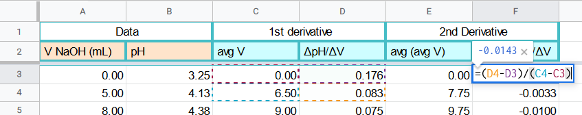
Second Derivative
The second derivative will follow the exact same steps as the first derivative. We now want to calculate the slope between each set of two data points form the first derivative. You will use the same formula but now applying it to the 1st derivative values
This can be done in google sheets using formulas
Average V
Since we used two data points to calculate the slope, we now need the average volume between those two points.
=AVERAGE(C3:C4)
Before making your graphs scroll to the bottom of your data. Check the last rows of data points. Are all of your formulas using data or are some using empty rows? Delete any cells where the number is not valid. (You should end up with less rows of data points for each derivative)
Finding Ka
Use the first and second derivative to find your equivalence point. (Note not the point observed in lab) Enter the volume of base added at that point in your WA Calculations tab
Use that value to determine your half equivalence point
Find the pH value at your half equivalence point. Use this value to determine your pKa. Then solve for your Ka value.
Week 2
First and Second Derivative
Now if you were so determined you could repeat all of the steps from week one to create your first and second derivative graphs. But since we are using google sheets we can make our lives much easier. You can right click your tab for WADerivatives and select duplicate. Now just rename your tab and enter in this weeks data. The number of rows most likely will not match so you may have to adjust your formulas (deleting or extending the formulas)
Remember that each derivative should have one less data point!
If you made the range for the charts the entire column it should automatically update the chart for your new data.
Finding Molar Mass
Use the definition of equivalence point to determine the number of mols of our acid in solution. You will need the molarity of your titrant to do so. Then use your mass of the unknown that you weighed in the lab and the mols of acid to determine the molar mass. (If you are stuck take a look at the units!)
Finding Ka
The steps of finding Ka are the same as last week