
2.2: Solubility Lab
- Page ID
- 361533

\( \newcommand{\vecs}[1]{\overset { \scriptstyle \rightharpoonup} {\mathbf{#1}} } \)
\( \newcommand{\vecd}[1]{\overset{-\!-\!\rightharpoonup}{\vphantom{a}\smash {#1}}} \)
\( \newcommand{\id}{\mathrm{id}}\) \( \newcommand{\Span}{\mathrm{span}}\)
( \newcommand{\kernel}{\mathrm{null}\,}\) \( \newcommand{\range}{\mathrm{range}\,}\)
\( \newcommand{\RealPart}{\mathrm{Re}}\) \( \newcommand{\ImaginaryPart}{\mathrm{Im}}\)
\( \newcommand{\Argument}{\mathrm{Arg}}\) \( \newcommand{\norm}[1]{\| #1 \|}\)
\( \newcommand{\inner}[2]{\langle #1, #2 \rangle}\)
\( \newcommand{\Span}{\mathrm{span}}\)
\( \newcommand{\id}{\mathrm{id}}\)
\( \newcommand{\Span}{\mathrm{span}}\)
\( \newcommand{\kernel}{\mathrm{null}\,}\)
\( \newcommand{\range}{\mathrm{range}\,}\)
\( \newcommand{\RealPart}{\mathrm{Re}}\)
\( \newcommand{\ImaginaryPart}{\mathrm{Im}}\)
\( \newcommand{\Argument}{\mathrm{Arg}}\)
\( \newcommand{\norm}[1]{\| #1 \|}\)
\( \newcommand{\inner}[2]{\langle #1, #2 \rangle}\)
\( \newcommand{\Span}{\mathrm{span}}\) \( \newcommand{\AA}{\unicode[.8,0]{x212B}}\)
\( \newcommand{\vectorA}[1]{\vec{#1}} % arrow\)
\( \newcommand{\vectorAt}[1]{\vec{\text{#1}}} % arrow\)
\( \newcommand{\vectorB}[1]{\overset { \scriptstyle \rightharpoonup} {\mathbf{#1}} } \)
\( \newcommand{\vectorC}[1]{\textbf{#1}} \)
\( \newcommand{\vectorD}[1]{\overrightarrow{#1}} \)
\( \newcommand{\vectorDt}[1]{\overrightarrow{\text{#1}}} \)
\( \newcommand{\vectE}[1]{\overset{-\!-\!\rightharpoonup}{\vphantom{a}\smash{\mathbf {#1}}}} \)
\( \newcommand{\vecs}[1]{\overset { \scriptstyle \rightharpoonup} {\mathbf{#1}} } \)
\( \newcommand{\vecd}[1]{\overset{-\!-\!\rightharpoonup}{\vphantom{a}\smash {#1}}} \)
\(\newcommand{\avec}{\mathbf a}\) \(\newcommand{\bvec}{\mathbf b}\) \(\newcommand{\cvec}{\mathbf c}\) \(\newcommand{\dvec}{\mathbf d}\) \(\newcommand{\dtil}{\widetilde{\mathbf d}}\) \(\newcommand{\evec}{\mathbf e}\) \(\newcommand{\fvec}{\mathbf f}\) \(\newcommand{\nvec}{\mathbf n}\) \(\newcommand{\pvec}{\mathbf p}\) \(\newcommand{\qvec}{\mathbf q}\) \(\newcommand{\svec}{\mathbf s}\) \(\newcommand{\tvec}{\mathbf t}\) \(\newcommand{\uvec}{\mathbf u}\) \(\newcommand{\vvec}{\mathbf v}\) \(\newcommand{\wvec}{\mathbf w}\) \(\newcommand{\xvec}{\mathbf x}\) \(\newcommand{\yvec}{\mathbf y}\) \(\newcommand{\zvec}{\mathbf z}\) \(\newcommand{\rvec}{\mathbf r}\) \(\newcommand{\mvec}{\mathbf m}\) \(\newcommand{\zerovec}{\mathbf 0}\) \(\newcommand{\onevec}{\mathbf 1}\) \(\newcommand{\real}{\mathbb R}\) \(\newcommand{\twovec}[2]{\left[\begin{array}{r}#1 \\ #2 \end{array}\right]}\) \(\newcommand{\ctwovec}[2]{\left[\begin{array}{c}#1 \\ #2 \end{array}\right]}\) \(\newcommand{\threevec}[3]{\left[\begin{array}{r}#1 \\ #2 \\ #3 \end{array}\right]}\) \(\newcommand{\cthreevec}[3]{\left[\begin{array}{c}#1 \\ #2 \\ #3 \end{array}\right]}\) \(\newcommand{\fourvec}[4]{\left[\begin{array}{r}#1 \\ #2 \\ #3 \\ #4 \end{array}\right]}\) \(\newcommand{\cfourvec}[4]{\left[\begin{array}{c}#1 \\ #2 \\ #3 \\ #4 \end{array}\right]}\) \(\newcommand{\fivevec}[5]{\left[\begin{array}{r}#1 \\ #2 \\ #3 \\ #4 \\ #5 \\ \end{array}\right]}\) \(\newcommand{\cfivevec}[5]{\left[\begin{array}{c}#1 \\ #2 \\ #3 \\ #4 \\ #5 \\ \end{array}\right]}\) \(\newcommand{\mattwo}[4]{\left[\begin{array}{rr}#1 \amp #2 \\ #3 \amp #4 \\ \end{array}\right]}\) \(\newcommand{\laspan}[1]{\text{Span}\{#1\}}\) \(\newcommand{\bcal}{\cal B}\) \(\newcommand{\ccal}{\cal C}\) \(\newcommand{\scal}{\cal S}\) \(\newcommand{\wcal}{\cal W}\) \(\newcommand{\ecal}{\cal E}\) \(\newcommand{\coords}[2]{\left\{#1\right\}_{#2}}\) \(\newcommand{\gray}[1]{\color{gray}{#1}}\) \(\newcommand{\lgray}[1]{\color{lightgray}{#1}}\) \(\newcommand{\rank}{\operatorname{rank}}\) \(\newcommand{\row}{\text{Row}}\) \(\newcommand{\col}{\text{Col}}\) \(\renewcommand{\row}{\text{Row}}\) \(\newcommand{\nul}{\text{Nul}}\) \(\newcommand{\var}{\text{Var}}\) \(\newcommand{\corr}{\text{corr}}\) \(\newcommand{\len}[1]{\left|#1\right|}\) \(\newcommand{\bbar}{\overline{\bvec}}\) \(\newcommand{\bhat}{\widehat{\bvec}}\) \(\newcommand{\bperp}{\bvec^\perp}\) \(\newcommand{\xhat}{\widehat{\xvec}}\) \(\newcommand{\vhat}{\widehat{\vvec}}\) \(\newcommand{\uhat}{\widehat{\uvec}}\) \(\newcommand{\what}{\widehat{\wvec}}\) \(\newcommand{\Sighat}{\widehat{\Sigma}}\) \(\newcommand{\lt}{<}\) \(\newcommand{\gt}{>}\) \(\newcommand{\amp}{&}\) \(\definecolor{fillinmathshade}{gray}{0.9}\)
Learning Objectives
Goals:
- Collect experimental data and create a solubility curve.
By the end of this lab, students should be able to:
- Properly use an analytical balance to measure mass.
- Set up an experimental work station to measure the solubility of a salt in water as a function of the temperature.
- Generate a Workbook using Google Sheets.
Prior knowledge:
Safety
- Emergency Preparedness
- Eye protection is mandatory in this lab, and you should not wear shorts or open toed shoes.
- KClO3 PubChem LCSS
- Minimize Risk
- Check the cord on the hotplate, inform the instructor if it is frayed.
- Make sure the electrical cord never touches the surface of the hotplate
- Recognize Hazards
- You will be working with an alcohol thermometer and care must be taken when handling it. You will be using a water bath to heat your solution and must always take care not to let the thermometer touch the bottom of the glass where it is in contact with the hot plate.
- All waste is placed in the labeled container in the hood and will be recycled when the lab is over. Contact your instructor if the waste container is full, or about full.
Please see UPenn EHRS Hot Plate Malfunctions and Misuse site for more information on accidents involving hot plates.
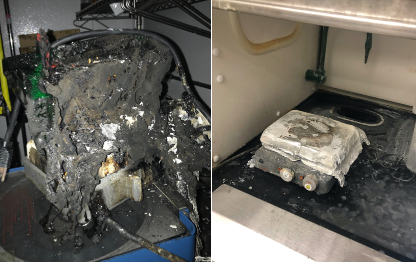 Figure \(\PageIndex{1}\): The hotplate on the left shows the aftermath of a fire when when a non-heat resistant container was placed on a hotplate. The worker thought they were only using the magnetic stirrer. (2021) The hot plate on the right should be discarded (CC0)
Equipment and materials needed
| 5 mL pipette and bulb | 500 mL beaker | 250 ml beaker |
| 8 in test tube | Thermometer | Wire Stirrer |
| Cork for 8 in test tube w/slot for stirrer and thermometer | Test tube clamp | Ring stand |
| 5 small test tubes and rack | analytical balance | Hot plate |
| KClO3(s) | Ice |
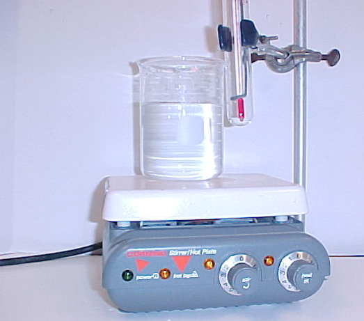
Figure \(\PageIndex{2}\): Experimental setup. See how the thermometer goes through the stirrer. When placing the test tube into the water bath do not have it touch the bottom, but add enough water to the bath so that it goes up to about an 2 inches from the top when the thermometer is inserted. (Copyright; Belford CC-BY)
Background
We are dissolving a salt in water and like most (not all) salts the solubility increases when the temperature increases and you need to figure out the concentration of a saturated solution as a function of the temperature, make 5 measurements and plot them. In each measurement you mix known masses of the salt and the water.
Problem 1: Figure \(\PageIndex{2}\)(a) is reading the temperature of a saturated solution, the problem is we do not know the concentration of the salt that dissolved. That is, the total salt added is the mass of the salt dissolved and the mass of the precipitate.
\[m_{Total \; Salt} = m_{Dissolved \; Salt} \; + \; m_{Precipitated \; Salt}\]
So even though the solution is saturated, we do no know its concentration of the solution, only the total concentration.
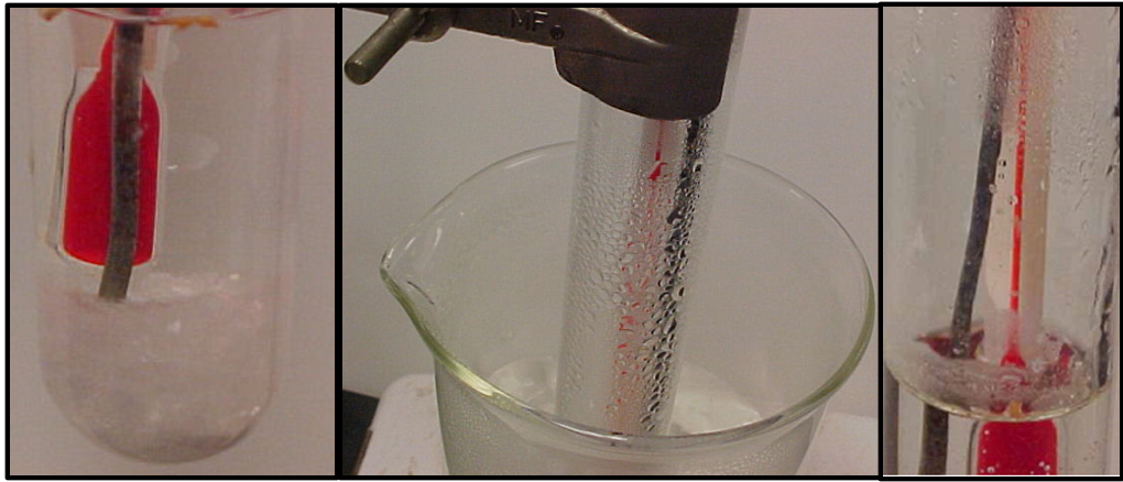 Figure \(\PageIndex{3}\): (a) left image shows a saturated solution with precipitate on the bottom, (b) middle image shows refluxing that can occur for high temperatures and (c) shows crystals forming where the cooler condensed water from the refluxing flows down the tube and hits the hotter water. (Copyright; Belford CC-BY)
Problem 2: Figure\(\PageIndex{2}\)(b) shows refluxing where hot water vapor rises up inside the test tube and hits the colder glass surface that is exposed to the air and condenses. When enough condensed water forms it flows back into the solution. When this cooler water hits the bulk hot water it cools it down, figure \(\PageIndex{2}\)(c), the solubility goes down and crystals form in a ring on the surface of the test tube at the interface of the hot liquid and the air. These crystals are a false reading and due to a temperature gradient, and we do not know the temperature that they were formed at, just that it is colder than the bulk temperature, which is the temperature the thermometer is reading.
Further reading on Experimental Design Considerations in 2.5: Solubility Resources
In this experiment you will need a solution that is 28% solute by weight. This is the mass of the solute divided by the total mass of solution
\[\%Salt=\frac{m_{salt}}{m_{salt}+m_{water}}(100)\]
Experimental Procedures
Teams of 2-3 individuals will work cooperatively to perform this experiment and fill out the solubility lab datasheet. Before leaving the lab they need to write their name on the sheet and get the instructor's dated signature. The instructor needs to take a photo of a completed datasheet before group members leave.
- Weigh about 4.2 grams of KClO3 record this mass to the 0.0001 g in your datasheet.
- Quantitatively transfer the KClO3 to the 8 inch test tube
- Calculate the volume of DI (Deionized) water you would need to add to that mass to make a solution that is approximately 28% KClO3 by mass. Assume the density of water to be 1.000 g/mL.
- Using a burette transfer around that volume of water to the 8 in test tube containing the KClO3. Record in the datasheet the exact volume of water transferred.
- Place the four small test tubes in a rack,
- wet them with DI
- empty them like you would if you were pouring them into the large test tube
- fill a 250 mL about 70% full with DI water
- using a 5 mL pipette transfer 5.00 mL of the DI water from the beaker to each test tube in the rack.
- Place about 300 ml of water in a 500 mL beaker and heat to approximately 90o C. Make sure to inspect the electrical line and keep it from touching the hot surface. You will use this water bath to heat your solution.
- Place a notched stopper through which is suspended a thermometer probe and a wire stirrer, into the mouth of the test tube as shown in figures \(\PageIndex{1}\) and \(\PageIndex{4}\). Lower the tube into the hot water bath and stir the contents with the wire stirrer until the crystals have all dissolved. Remove the tube from the water bath and allow the contents to cool while continuing to stir the mixture. Carefully observe the contents of the tube while cooling is occurring and note and record the temperature at which crystals first appear.
 Figure \(\PageIndex{4}\): Solubility apparatus setup. (Copyright; Belford CC-BY)
- Add additional 5 mL of water and continue cooling if crystals dissolve upon dilution. If they do not dissolve, place back in water bath until they dissolve. If you do this step rapidly the solution will not have cooled enough to be saturated and they will not need to be reheated.
- Repeat steps 5 and 6 until you have recorded data for a total of 5 solutions, recording all values in your data sheet.
Data Analysis
The link to make a copy of the template is located on the next page
Remember to fill out the google form to link your workbook to the instructor.
Cover Sheet
The first sheet of your Workbook is always your cover page. You will paste your three graphs here when you are done.
 Figure \(\PageIndex{5}\): Cover Page. (Copyright; Belford CC 0.0)
Data Sheet
The second sheet will be where you work up your data. Copy the raw data from the datasheet you used in class and enter it into the "orange" cells. Then perform the calculations in the blue cells. You must put your answers in this table, as it is connected to the grader's workbook. If you choose, you can use functions in this sheet, or you can do the calculations by hand. The last column is for Units, pay attention to Column A as it specifies which units certain values should be in.
 Figure \(\PageIndex{6}\): Data Page. (Copyright; Belford CC 0.0)
NOTE: Throughout the semester we will color code the sheets, and all cells with a color are connected to your grader's workbook, and so you need to place something in them for full credit.
Data Input:
Input Data from your data sheet to the precision recorded in the lab.
Tutorial: Format Numbers and Decimal Places in google sheets
Mass Solid: The mass you actually weighed out in lab. What measuring device did we use? What is the precision for that device? Did the mass change throughout the experiment?
Water added: The amount of water added for each step. What did we use to measure the water? What is the precision for that device? What unit is it in?
Temp Crystals: What temperature did the crystals form for that solution? What measuring device did we use? What is the precision for that device?
Name Salt: Identify the name of the salt used for this experiment
Molar Mass Salt: What is the molar mass of the salt used for this experiment? What Unit is molar mass?
Calculations:
Now its time to do some calculations using your data. Its recommended to work out the calculation for solution 1 first on paper then you can turn it into a formula to repeat for the other solutions.
Tutorial: Basic Data Manipulations and Using Formulas to automate calculations
Total mL of water: Use the water added from above to find the total amount of water present in the solution at this step
Conc (g/100g H2O): Find the concentration of the solution in the units grams of salt per 100g of water. What is the difference between g/g H2O and g/100g H2O?
The density of pure water is 1g=1mL. Why do we specify pure water here?
Mass % salt: The mass percent in terms of the salt. Mass %= mass solute/ mass of solution
Molality: Find the concentration of the solution in units of molality. m=molality=mol solute/kg solvent
Mole Fraction salt: Find the mole fraction of salt in the solution. x=mol fraction=mol solute/mols of solution
Remember to report all values with the proper significant figures and include the appropriate units in column G
Graph Sheet
In this sheet you will insert a chart with a graph
In the previous lab 1: Graphing we learned how to make charts with labels and use a trendline to find the equation.
Chart 1: Linear Function
First make a graph of the solubility (g salt/100 g H2O) as a function of temperature.
Design Requirement
- Smoothline chart with dashed lines and data points
- This is the same design as the multiple series chart in the graphing lab, though now only with one set of data.
Insert a trendline and show a linear equation and the R2 value. How well does the line fit this data?
Chart 2: Power Function
Next copy the chart then show a power series equation and the R2 value. What changed? Did the R2 value increase or decrease?
Chart 3: Exponential Function
Copy the chart again and show an exponential equation and the R2 value. What is the R2 value now?
Of all the graphs, which fit is best?
Remember to copy and paste your charts to the coverpage
Coverpage: Saturation Label
The last part of the lab is to label undersaturated, saturated, and supersaturated.
On the coverpage click on the label in the box. Then click and drag it to the appropriate spot on the first chart, Solubility Curve Linear Function.
On some browsers the chart is set to always be on top and the labels will automatically be hidden by the chart
If so you can make the background transparent to avoid the issue

Make sure that link sharing is on and you've entered it to the google form!