
2: Thermogravimetry
- Page ID
- 476293

\( \newcommand{\vecs}[1]{\overset { \scriptstyle \rightharpoonup} {\mathbf{#1}} } \)
\( \newcommand{\vecd}[1]{\overset{-\!-\!\rightharpoonup}{\vphantom{a}\smash {#1}}} \)
\( \newcommand{\dsum}{\displaystyle\sum\limits} \)
\( \newcommand{\dint}{\displaystyle\int\limits} \)
\( \newcommand{\dlim}{\displaystyle\lim\limits} \)
\( \newcommand{\id}{\mathrm{id}}\) \( \newcommand{\Span}{\mathrm{span}}\)
( \newcommand{\kernel}{\mathrm{null}\,}\) \( \newcommand{\range}{\mathrm{range}\,}\)
\( \newcommand{\RealPart}{\mathrm{Re}}\) \( \newcommand{\ImaginaryPart}{\mathrm{Im}}\)
\( \newcommand{\Argument}{\mathrm{Arg}}\) \( \newcommand{\norm}[1]{\| #1 \|}\)
\( \newcommand{\inner}[2]{\langle #1, #2 \rangle}\)
\( \newcommand{\Span}{\mathrm{span}}\)
\( \newcommand{\id}{\mathrm{id}}\)
\( \newcommand{\Span}{\mathrm{span}}\)
\( \newcommand{\kernel}{\mathrm{null}\,}\)
\( \newcommand{\range}{\mathrm{range}\,}\)
\( \newcommand{\RealPart}{\mathrm{Re}}\)
\( \newcommand{\ImaginaryPart}{\mathrm{Im}}\)
\( \newcommand{\Argument}{\mathrm{Arg}}\)
\( \newcommand{\norm}[1]{\| #1 \|}\)
\( \newcommand{\inner}[2]{\langle #1, #2 \rangle}\)
\( \newcommand{\Span}{\mathrm{span}}\) \( \newcommand{\AA}{\unicode[.8,0]{x212B}}\)
\( \newcommand{\vectorA}[1]{\vec{#1}} % arrow\)
\( \newcommand{\vectorAt}[1]{\vec{\text{#1}}} % arrow\)
\( \newcommand{\vectorB}[1]{\overset { \scriptstyle \rightharpoonup} {\mathbf{#1}} } \)
\( \newcommand{\vectorC}[1]{\textbf{#1}} \)
\( \newcommand{\vectorD}[1]{\overrightarrow{#1}} \)
\( \newcommand{\vectorDt}[1]{\overrightarrow{\text{#1}}} \)
\( \newcommand{\vectE}[1]{\overset{-\!-\!\rightharpoonup}{\vphantom{a}\smash{\mathbf {#1}}}} \)
\( \newcommand{\vecs}[1]{\overset { \scriptstyle \rightharpoonup} {\mathbf{#1}} } \)
\(\newcommand{\longvect}{\overrightarrow}\)
\( \newcommand{\vecd}[1]{\overset{-\!-\!\rightharpoonup}{\vphantom{a}\smash {#1}}} \)
\(\newcommand{\avec}{\mathbf a}\) \(\newcommand{\bvec}{\mathbf b}\) \(\newcommand{\cvec}{\mathbf c}\) \(\newcommand{\dvec}{\mathbf d}\) \(\newcommand{\dtil}{\widetilde{\mathbf d}}\) \(\newcommand{\evec}{\mathbf e}\) \(\newcommand{\fvec}{\mathbf f}\) \(\newcommand{\nvec}{\mathbf n}\) \(\newcommand{\pvec}{\mathbf p}\) \(\newcommand{\qvec}{\mathbf q}\) \(\newcommand{\svec}{\mathbf s}\) \(\newcommand{\tvec}{\mathbf t}\) \(\newcommand{\uvec}{\mathbf u}\) \(\newcommand{\vvec}{\mathbf v}\) \(\newcommand{\wvec}{\mathbf w}\) \(\newcommand{\xvec}{\mathbf x}\) \(\newcommand{\yvec}{\mathbf y}\) \(\newcommand{\zvec}{\mathbf z}\) \(\newcommand{\rvec}{\mathbf r}\) \(\newcommand{\mvec}{\mathbf m}\) \(\newcommand{\zerovec}{\mathbf 0}\) \(\newcommand{\onevec}{\mathbf 1}\) \(\newcommand{\real}{\mathbb R}\) \(\newcommand{\twovec}[2]{\left[\begin{array}{r}#1 \\ #2 \end{array}\right]}\) \(\newcommand{\ctwovec}[2]{\left[\begin{array}{c}#1 \\ #2 \end{array}\right]}\) \(\newcommand{\threevec}[3]{\left[\begin{array}{r}#1 \\ #2 \\ #3 \end{array}\right]}\) \(\newcommand{\cthreevec}[3]{\left[\begin{array}{c}#1 \\ #2 \\ #3 \end{array}\right]}\) \(\newcommand{\fourvec}[4]{\left[\begin{array}{r}#1 \\ #2 \\ #3 \\ #4 \end{array}\right]}\) \(\newcommand{\cfourvec}[4]{\left[\begin{array}{c}#1 \\ #2 \\ #3 \\ #4 \end{array}\right]}\) \(\newcommand{\fivevec}[5]{\left[\begin{array}{r}#1 \\ #2 \\ #3 \\ #4 \\ #5 \\ \end{array}\right]}\) \(\newcommand{\cfivevec}[5]{\left[\begin{array}{c}#1 \\ #2 \\ #3 \\ #4 \\ #5 \\ \end{array}\right]}\) \(\newcommand{\mattwo}[4]{\left[\begin{array}{rr}#1 \amp #2 \\ #3 \amp #4 \\ \end{array}\right]}\) \(\newcommand{\laspan}[1]{\text{Span}\{#1\}}\) \(\newcommand{\bcal}{\cal B}\) \(\newcommand{\ccal}{\cal C}\) \(\newcommand{\scal}{\cal S}\) \(\newcommand{\wcal}{\cal W}\) \(\newcommand{\ecal}{\cal E}\) \(\newcommand{\coords}[2]{\left\{#1\right\}_{#2}}\) \(\newcommand{\gray}[1]{\color{gray}{#1}}\) \(\newcommand{\lgray}[1]{\color{lightgray}{#1}}\) \(\newcommand{\rank}{\operatorname{rank}}\) \(\newcommand{\row}{\text{Row}}\) \(\newcommand{\col}{\text{Col}}\) \(\renewcommand{\row}{\text{Row}}\) \(\newcommand{\nul}{\text{Nul}}\) \(\newcommand{\var}{\text{Var}}\) \(\newcommand{\corr}{\text{corr}}\) \(\newcommand{\len}[1]{\left|#1\right|}\) \(\newcommand{\bbar}{\overline{\bvec}}\) \(\newcommand{\bhat}{\widehat{\bvec}}\) \(\newcommand{\bperp}{\bvec^\perp}\) \(\newcommand{\xhat}{\widehat{\xvec}}\) \(\newcommand{\vhat}{\widehat{\vvec}}\) \(\newcommand{\uhat}{\widehat{\uvec}}\) \(\newcommand{\what}{\widehat{\wvec}}\) \(\newcommand{\Sighat}{\widehat{\Sigma}}\) \(\newcommand{\lt}{<}\) \(\newcommand{\gt}{>}\) \(\newcommand{\amp}{&}\) \(\definecolor{fillinmathshade}{gray}{0.9}\)After completing this chapter, you should be able to:
- Describe the effect of heat on materials.
- Identify physical and chemical transitions.
- Describe the essential features of a thermobalance.
- Draw and interpret thermogravimetric and derivative thermogravimetric curve for a known system.
- Illustrate the range of applications of thermogravimetry.
- Calculate % weight loss at every stage of decomposition and predict stoichiometry.
Thermogravimetry is a technique used to detect any physical or chemical transitions which are accompanied by a weight loss or weight gain as the sample is heated in a controlled manner.
2.1 Effect of heat on matter
We need to first understand the effects of heat on matter. And For further explanation please see Introductory Chemistry in Libretexts
Now, we have understood the effects of heat on matter and also able to identify the processes involving change in weight on heating through Activity 1D. It is important to keep in mind that the change in weight could be due to physical or chemical transitions. To be able to distinguish between physical and chemical transition, let us go through the next sub-topic.
2.2 Changes in matter: Physical and Chemical Changes
For further explanation please see Introductory Chemistry in Libretexts
Activity 2.1: Can you assign which of these transitions will be physical transitions /chemical transitions? (please tick)
| Phenomenon | Physical | Chemical |
|---|---|---|
| Adsorption | ||
| Dehydration | ||
| Desorption | ||
| Fusion (melting) | ||
| Chemisorption | ||
| Vaporization | ||
| Decomposition | ||
| Redox reactions | ||
| Reduction in gaseous atmosphere |
(Dodd & Tonge, 2008)
2.3 Principle and Instrumentation of TGA
The instrument used to carry out thermogravimetric analysis is known as “thermobalance”.
Working: Please go through the Chemlibre link to understand the principle and working of a thermobalance.
2.4 Interpretation of thermogravimetric curve
The graphical information obtained from thermogravimetric analysis is known as thermogram/pyrolysis curve. TG curve is a plot of weight (W) decreasing downwards on the y-axis (ordinate), and temperature (T) increasing to the right on the x-axis (abscissa). A typical thermogram for a single step decomposition is shown in Fig. 2.4.
The plateau ‘AB’ indicates no change in weight or the temperature range over which the sample is thermally stable. At point ‘B’ the sample starts decomposing which is indicated by an inflexion.
Please read the following text explaining the interpretation of thermogram and then attempt Activity 2B.
Activity 2.2: A typical thermogram is shown below, observe and fill in the blanks by choosing the most appropriate answer. (Hint: Initial mass at ‘A’ is considered as 100%)

Query \(\Page}\)
Activity 2.3: For the processes given in the table, predict the nature of thermogram (Type-X /Type-Y or None of these)
| Phenomenon | Type | 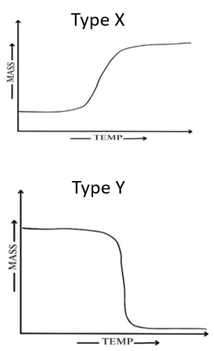 |
| Melting | ||
| Adsorption of gas | ||
| Desorption of gas | ||
| Vaporisation | ||
| Dehydration | ||
| Decomposition | ||
| Sublimation |
2.5 Need for Derivative Thermogravimetry (DTG)
In the above example (Fig. 2.4), we have considered the thermogravimetric curve which represents a single stage decomposition. Figures ‘1.2.5a’ and ‘1.2.5b’ show two-stage and three-stage decompositions respectively. In both these figures (2.5a and 2.5b) there is an overlay of TGA and DTG thermograms, clearly depicting advantages of DTG over TGA thermogram in locating the exact decomposition temperature.

Figure 2.5a. Thermogravimetric (TG) and Derivative thermogravimetry (DTG) curves for PVP at a heating rate of 10°C/min. (Source: Al-Hada et al., 2014) https://images.app.goo.gl/fWChwNJi9uxfHZAJ7
Figure ‘2.5b’ is for the decomposition of calcium oxalate monohydrate, the weight loss commences just above 100°C and continues up to 200°C. Between about 400 °C and 500°C further decomposition occurs, to give a product which is stable up to 700°C before decomposing to give another stable compound at 800°C. Every process of decomposition continues over a range of temperature hence the DTG curve is useful in providing information regarding precise decomposition temperature at every stage.
Activity 2.4: (James & Tonge, 2008)
Activity 2.5: Complete the following reaction for the decomposition of calcium carbonate.
- Identify the volatile and stable compound/s remaining in the crucible post decomposition and indicate these on a thermogram.

Activity 2.6: Observe the image given below for the decomposition of magnesium oxalate monohydrate (MgC2O4.H2O)and complete the activity.
- Identify the volatile product and the residue remaining in the crucible at each stage of decomposition.
- Write the decomposition reaction taking place at each stage.
- Draw a thermogram for the decomposition of magnesium oxalate monohydrate.

Activity 2.7: Observe the image given below for the decomposition of ammonium nitrate (NH4NO3) and complete the activity.
- Identify the volatile product/s and the residue remaining (if any) in the crucible after decomposition.
- Write the decomposition reaction.
- Draw a thermogram for the decomposition of ammonium nitrate.
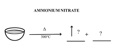
i. Compare ammonium nitrate decomposition curve obtained in Activity 2.7 with calcium carbonate thermogram obtained in Activity 2.5
ii. Can you suggest why ammonium nitrate thermogram shows zero mass post decomposition?
2.6 Applications of Thermogravimetric analysis
I. Thermogravimetric analysis of a binary mixture of calcium and magnesium oxalates:
Following thermogram shows decomposition curve for a mixture of oxalates.
- There is a significant loss which occurs before 210°C- due to loss of water from the sample.
- The mixture of anhydrous carbonate then shows some weight loss by about 480 °C owing to the reaction
MgCO3(s) → MgO (s) + CO2 (g)
- No further weight loss occurs before 600 °C. (EF)
- CaCO3 decomposes between about 600 °C and 900 °C. (FG)
CaCO3 (s) → CaO (s) + CO2 (g)
- Thus, EF represents a mixture of MgO and CaCO3
- The plateau GH represents the residue of MgO and CaO
Activity 2.8: Construct separate decomposition curves for calcium oxalate dihydrate and magnesium oxalate dihydrate based on the above information.
II. Thermogravimetric analysis of plaster for safety screening:
Plaster contains following ingredients,
Gypsum--- CaSO4.2H2O
Lime--- Ca(OH)2
Chalk--- CaCO3
From the weight loss at each step on the curve, the quantity of each ingredient can be determined in the original sample. In the manufacture of Portland cement, 5% gypsum is added to reduce the rate of setting. The gypsum is added to the fused clinker during processing, and the two components are subsequently milled to obtain uniform mixing and the required particle size. During milling, the thermal energy generated may cause partial dehydration of gypsum to hemihydrate CaSO4 .1/2 H2O which adversely affects (increases) the rate of setting of the cement. Hence it is important to monitor the presence of each hydrate in the final cement. In order to provide quantitation at the required levels, this problem can be solved by TGA and DTA or DSC.
The dehydration of gypsum occurs as a two-stage endothermic process.
CaSO4.2H2O → CaSO4.1/2 H2O → CaSO4
So, if there is conversion of gypsum to hemihydrate, the TG curve in Fig. 2.6b will show two step decomposition for gypsum instead of one.
Draw a TG curve for plaster in which the gypsum is converted into a hemihydrate form.
Activity 2.9: (James &Tonge, 2008)
A manufacturer wishes to incorporate a plastic coating on the inside of a utensil. One factor to be evaluated is the stability of the following polymer.
a. Polyethylene
b. Polypropylene
c. PVC
d. Polytetrafluoroethylene
Figure below gives TG curves for the above polymers.

So far, we have discussed qualitative applications of TGA. Let us see some quantitative applications of thermogravimetric measurement.
Activity 2.10: Solve the following numerical problems.
1) Calculate the percent weight changes W% for each of the following reactions which occur on heating the parent material.
a) Ca(OH)2(S) →CaO (s) +H2O(g)
b) 6PbO(s) + O2(g) → 2Pb3O4(s)
[Ca=40.1, H=1.0, O=16.0, Pb=207.2]
2) A mixture of calcium oxide and calcium carbonate is analysed by thermogravimetry. The resultant curve indicates one decomposition only between 600-900° C during which the weight of sample decreases from 250.6 mg to 190.8 mg. What is the percentage of calcium carbonate in mixture by weight?
[Atomic mass: H=1.0, Pb=207.2, C=12.0, O=16.0, Ca= 40.1]
3) The thermogram given below shows the mass of a sample of calcium oxalate monohydrate, CaC2O4.H2O, as a function of temperature. The original sample of 17.61 mg was heated from room temperature to 1000°C at a rate of 20°C per minute. Calculate the % weight loss at each step.
For the TG curve shown in Numerical-3,
i. Write the decomposition reaction at each step.
ii. Identify the volatilization product and the solid residue that remains at every step.
Activity 2.11: Solve the puzzle