31.1: Thermogravimetry

One method for determining the products of a thermal decomposition is to monitor the sample’s mass as a function of temperature, a process called a thermogravimetric analysis (TGA) or thermogravimetry. Figure 31.1.1 shows a typical thermogram in which each change in mass—each “step” in the thermogram—represents the loss of a volatile product. As the following example illustrates, we can use a thermogram to identify a compound’s decomposition reactions.

Figure 31.1.1 . Thermogram for CaC₂O₄•H₂O obtained by heating a sample from room temperature to 1000^oC at a rate of 20^oC/min. Each change in mass results from the loss of a volatile product. The sample’s initial mass and its mass after each loss are shown by the dotted lines. See Example 31.1.1 for information on interpreting this thermogram.

Example 31.1.1

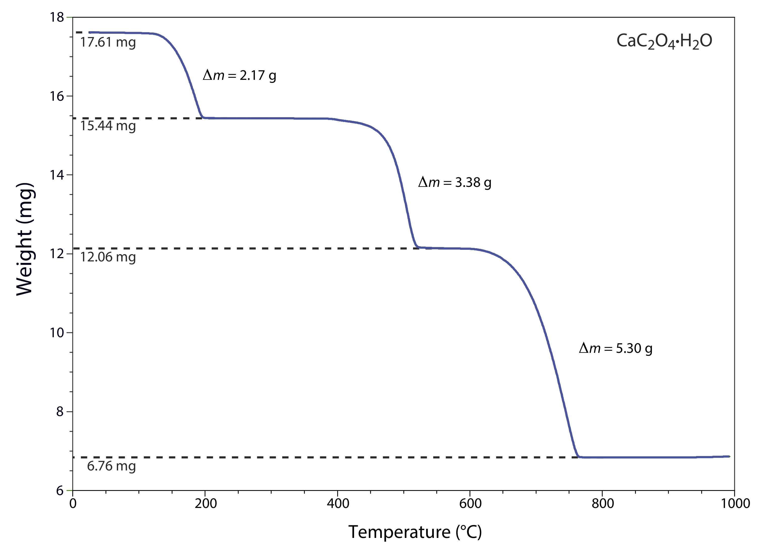
The thermogram in Figure 31.1.1 shows the mass of a sample of calcium oxalate monohydrate, CaC₂O₄•H₂O, as a function of temperature. The original sample of 17.61 mg was heated from room temperature to 1000^oC at a rate of 20^oC per minute. For each step in the thermogram, identify the volatilization product and the solid residue that remains.

Solution

From 100–250^oC the sample loses 17.61 mg – 15.44 mg, or 2.17 mg, which is

\[\frac{2.17 \ \mathrm{mg}}{17.61 \ \mathrm{mg}} \times 100=12.3 \% \nonumber \]

of the sample’s original mass. In terms of CaC₂O₄•H₂O, this corresponds to a decrease in the molar mass of

\[0.123 \times 146.11 \ \mathrm{g} / \mathrm{mol}=18.0 \ \mathrm{g} / \mathrm{mol} \nonumber \]

The product’s molar mass and the temperature range for the decomposition, suggest that this is a loss of H₂O(g), leaving a residue of CaC₂O₄.

The loss of 3.38 mg from 350–550^oC is a 19.2% decrease in the sample’s original mass, or a decrease in the molar mass of

\[0.192 \times 146.11 \ \mathrm{g} / \mathrm{mol}=28.1 \ \mathrm{g} / \mathrm{mol} \nonumber \]

which is consistent with the loss of CO(g) and a residue of CaCO₃.

Finally, the loss of 5.30 mg from 600-800^oC is a 30.1% decrease in the sample’s original mass, or a decrease in molar mass of

\[0.301 \times 146.11 \ \mathrm{g} / \mathrm{mol}=44.0 \ \mathrm{g} / \mathrm{mol} \nonumber \]

This loss in molar mass is consistent with the release of CO₂(g), leaving a final residue of CaO. The three decomposition reactions are

\[\begin{array}{c}{\mathrm{CaC}_{2} \mathrm{O}_{4} \cdot \mathrm{H}_{2} \mathrm{O}(s) \rightarrow \ \mathrm{CaC}_{2} \mathrm{O}_{4}(s)+2 \mathrm{H}_{2} \mathrm{O}(l)} \\ {\mathrm{CaC}_{2} \mathrm{O}_{4}(s) \rightarrow \ \mathrm{CaCO}_{3}(s)+\mathrm{CO}(g)} \\ {\mathrm{CaCO}_{3}(s) \rightarrow \ \mathrm{CaO}(s)+\mathrm{CO}_{2}(g)}\end{array} \nonumber \]

Identifying the products of a thermal decomposition provides information that we can use to develop an analytical procedure. For example, the thermogram in Figure 31.1.1 shows that we must heat a precipitate of CaC₂O₄•H₂O to a temperature between 250 and 400^oC if we wish to isolate and weigh CaC₂O₄. Alternatively, heating the sample to 1000^oC allows us to isolate and weigh CaO.

Exercise 31.1.1

Under the same conditions as Figure 31.1.1 , the thermogram for a 22.16 mg sample of MgC₂O₄•H₂O shows two steps: a loss of 3.06 mg from 100–250^oC and a loss of 12.24 mg from 350–550^oC. For each step, identify the volatilization product and the solid residue that remains. Using your results from this exercise and the results from Example 31.1.1 , explain how you can use thermogravimetry to analyze a mixture that contains CaC₂O₄•H₂O and MgC₂O₄•H₂O. You may assume that other components in the sample are inert and thermally stable below 1000^oC.

Answer

From 100–250^oC the sample loses 13.8% of its mass, or a loss of

\[0.138 \times 130.34 \ \mathrm{g} / \mathrm{mol}=18.0 \ \mathrm{g} / \mathrm{mol} \nonumber \]

which is consistent with the loss of H₂O(g) and a residue of MgC₂O₄.

From 350–550^oC the sample loses 55.23% of its original mass, or a loss of

\[0.5523 \times 130.34 \ \mathrm{g} / \mathrm{mol}=71.99 \ \mathrm{g} / \mathrm{mol} \nonumber \]

This weight loss is consistent with the simultaneous loss of CO(g) and CO₂(g), leaving a residue of MgO.

We can analyze the mixture by heating a portion of the sample to 300^oC, 600^oC, and 1000^oC, recording the mass at each temperature. The loss of mass between 600^oC and 1000^oC, \(\Delta m_2\), is due to the loss of CO₂(g) from the decomposition of CaCO₃ to CaO, and is proportional to the mass of CaC₂O₄•H₂O in the sample.

\[\mathrm{g} \ \mathrm{CaC}_{2} \mathrm{O}_{4} \cdot \mathrm{H}_{2} \mathrm{O}=\Delta m_{2} \times \frac{1 \ \mathrm{mol} \ \mathrm{CO}_{2}}{44.01 \ \mathrm{g} \ \mathrm{CO}_{2}} \times \frac{146.11 \ \mathrm{g} \ \mathrm{CaC}_{2} \mathrm{O}_{4} \cdot \mathrm{H}_{2} \mathrm{O}}{\mathrm{mol} \ \mathrm{CO}_{2}} \nonumber \]

The change in mass between 300^oC and 600^oC, \(\Delta m_1\), is due to the loss of CO(g) from CaC₂O₄•H₂O and the loss of CO(g) and CO₂(g) from MgC₂O₄•H₂O. Because we already know the amount of CaC₂O₄•H₂O in the sample, we can calculate its contribution to \(\Delta m_1\).

\[\left(\Delta m_{1}\right)_{\mathrm{Ca}}=\mathrm{g} \ \mathrm{CaC}_{2} \mathrm{O}_{4} \cdot \mathrm{H}_{2} \mathrm{O}=\Delta m_{2} \times \frac{1 \ \mathrm{mol} \ \mathrm{CO}}{146.11 \ \mathrm{g} \ \mathrm{CaC}_{2} \mathrm{O}_{4} \cdot \mathrm{H}_{2} \mathrm{O}} \times \frac{28.01 \ \mathrm{g} \ \mathrm{CO}}{\mathrm{mol} \ \mathrm{CO}} \nonumber \]

The change in mass between 300^oC and 600^oC due to the decomposition of MgC₂O₄•H₂O

\[\left(m_{1}\right)_{\mathrm{Mg}}=\Delta m_{1}-\left(\Delta m_{1}\right)_{\mathrm{Ca}} \nonumber \]

provides the mass of MgC₂O₄•H₂O in the sample.

\[\mathrm{g} \ \mathrm{MgC}_{2} \mathrm{O}_{4} \cdot \mathrm{H}_{2} \mathrm{O}=\left(\Delta m_{1}\right)_{\mathrm{Mg}} \times \frac{1 \ \mathrm{mol}\left(\mathrm{CO} \ + \ \mathrm{CO}_{2}\right)}{130.35 \ \mathrm{g} \ \mathrm{MgC}_{2} \mathrm{O}_{4} \cdot \mathrm{H}_{2} \mathrm{O}} \times \frac{78.02 \ \mathrm{g} \ \left(\mathrm{CO} \ + \ \mathrm{CO}_{2}\right)}{\mathrm{mol}\ \left(\mathrm{CO} \ + \ \mathrm{CO}_{2}\right)} \nonumber \]

Instrumentation

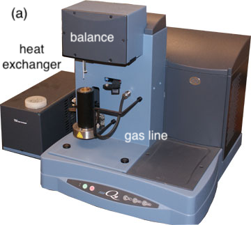
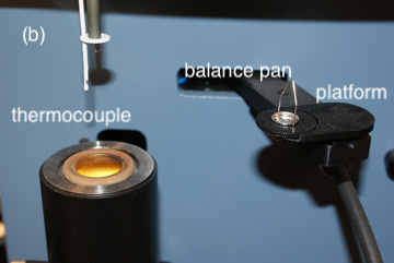
In a thermogravimetric analysis, the sample is placed on a small balance pan attached to one arm of an electromagnetic balance (Figure 31.1.2 ). The sample is lowered into an electric furnace and the furnace’s temperature is increased at a fixed rate of a few degrees per minute while monitoring continuously the sample’s weight. The instrument usually includes a gas line for purging the volatile decomposition products out of the furnace, and a heat exchanger to dissipate the heat emitted by the furnace.

Figure 31.1.2 . (a) Instrumentation for conducting a thermogravimetric analysis. The balance sits on the top of the instrument with the sample suspended below. A gas line supplies an inert gas that sweeps the volatile decomposition products out of the furnace. The heat exchanger dissipates the heat from the furnace to a reservoir of water. (b) Close-up showing the balance pan, which sits on a moving platform, the thermocouple for monitoring temperature, a hook for lowering the sample pan into the furnace, and the opening to the furnace. After placing a small portion of the sample on the balance pan, the platform rotates over the furnace and transfers the balance pan to a hook that is suspended from the balance. Once the balance pan is in place, the platform rotates back to its initial position. The balance pan and the thermocouple are then lowered into the furnace.

Applications

Perhaps the most important application gravimetry is exploring a compound's thermal stability, as illustrated in Figure \(\PageIndex{1}\) and Exercise \(\PageIndex{1}\) for calcium oxalate hydrate. TGA is particularly useful for studying the thermal stability of polymers.