
2: Density and Graphing
- Page ID
- 316197
\( \newcommand{\vecs}[1]{\overset { \scriptstyle \rightharpoonup} {\mathbf{#1}} } \)
\( \newcommand{\vecd}[1]{\overset{-\!-\!\rightharpoonup}{\vphantom{a}\smash {#1}}} \)
\( \newcommand{\dsum}{\displaystyle\sum\limits} \)
\( \newcommand{\dint}{\displaystyle\int\limits} \)
\( \newcommand{\dlim}{\displaystyle\lim\limits} \)
\( \newcommand{\id}{\mathrm{id}}\) \( \newcommand{\Span}{\mathrm{span}}\)
( \newcommand{\kernel}{\mathrm{null}\,}\) \( \newcommand{\range}{\mathrm{range}\,}\)
\( \newcommand{\RealPart}{\mathrm{Re}}\) \( \newcommand{\ImaginaryPart}{\mathrm{Im}}\)
\( \newcommand{\Argument}{\mathrm{Arg}}\) \( \newcommand{\norm}[1]{\| #1 \|}\)
\( \newcommand{\inner}[2]{\langle #1, #2 \rangle}\)
\( \newcommand{\Span}{\mathrm{span}}\)
\( \newcommand{\id}{\mathrm{id}}\)
\( \newcommand{\Span}{\mathrm{span}}\)
\( \newcommand{\kernel}{\mathrm{null}\,}\)
\( \newcommand{\range}{\mathrm{range}\,}\)
\( \newcommand{\RealPart}{\mathrm{Re}}\)
\( \newcommand{\ImaginaryPart}{\mathrm{Im}}\)
\( \newcommand{\Argument}{\mathrm{Arg}}\)
\( \newcommand{\norm}[1]{\| #1 \|}\)
\( \newcommand{\inner}[2]{\langle #1, #2 \rangle}\)
\( \newcommand{\Span}{\mathrm{span}}\) \( \newcommand{\AA}{\unicode[.8,0]{x212B}}\)
\( \newcommand{\vectorA}[1]{\vec{#1}} % arrow\)
\( \newcommand{\vectorAt}[1]{\vec{\text{#1}}} % arrow\)
\( \newcommand{\vectorB}[1]{\overset { \scriptstyle \rightharpoonup} {\mathbf{#1}} } \)
\( \newcommand{\vectorC}[1]{\textbf{#1}} \)
\( \newcommand{\vectorD}[1]{\overrightarrow{#1}} \)
\( \newcommand{\vectorDt}[1]{\overrightarrow{\text{#1}}} \)
\( \newcommand{\vectE}[1]{\overset{-\!-\!\rightharpoonup}{\vphantom{a}\smash{\mathbf {#1}}}} \)
\( \newcommand{\vecs}[1]{\overset { \scriptstyle \rightharpoonup} {\mathbf{#1}} } \)
\(\newcommand{\longvect}{\overrightarrow}\)
\( \newcommand{\vecd}[1]{\overset{-\!-\!\rightharpoonup}{\vphantom{a}\smash {#1}}} \)
\(\newcommand{\avec}{\mathbf a}\) \(\newcommand{\bvec}{\mathbf b}\) \(\newcommand{\cvec}{\mathbf c}\) \(\newcommand{\dvec}{\mathbf d}\) \(\newcommand{\dtil}{\widetilde{\mathbf d}}\) \(\newcommand{\evec}{\mathbf e}\) \(\newcommand{\fvec}{\mathbf f}\) \(\newcommand{\nvec}{\mathbf n}\) \(\newcommand{\pvec}{\mathbf p}\) \(\newcommand{\qvec}{\mathbf q}\) \(\newcommand{\svec}{\mathbf s}\) \(\newcommand{\tvec}{\mathbf t}\) \(\newcommand{\uvec}{\mathbf u}\) \(\newcommand{\vvec}{\mathbf v}\) \(\newcommand{\wvec}{\mathbf w}\) \(\newcommand{\xvec}{\mathbf x}\) \(\newcommand{\yvec}{\mathbf y}\) \(\newcommand{\zvec}{\mathbf z}\) \(\newcommand{\rvec}{\mathbf r}\) \(\newcommand{\mvec}{\mathbf m}\) \(\newcommand{\zerovec}{\mathbf 0}\) \(\newcommand{\onevec}{\mathbf 1}\) \(\newcommand{\real}{\mathbb R}\) \(\newcommand{\twovec}[2]{\left[\begin{array}{r}#1 \\ #2 \end{array}\right]}\) \(\newcommand{\ctwovec}[2]{\left[\begin{array}{c}#1 \\ #2 \end{array}\right]}\) \(\newcommand{\threevec}[3]{\left[\begin{array}{r}#1 \\ #2 \\ #3 \end{array}\right]}\) \(\newcommand{\cthreevec}[3]{\left[\begin{array}{c}#1 \\ #2 \\ #3 \end{array}\right]}\) \(\newcommand{\fourvec}[4]{\left[\begin{array}{r}#1 \\ #2 \\ #3 \\ #4 \end{array}\right]}\) \(\newcommand{\cfourvec}[4]{\left[\begin{array}{c}#1 \\ #2 \\ #3 \\ #4 \end{array}\right]}\) \(\newcommand{\fivevec}[5]{\left[\begin{array}{r}#1 \\ #2 \\ #3 \\ #4 \\ #5 \\ \end{array}\right]}\) \(\newcommand{\cfivevec}[5]{\left[\begin{array}{c}#1 \\ #2 \\ #3 \\ #4 \\ #5 \\ \end{array}\right]}\) \(\newcommand{\mattwo}[4]{\left[\begin{array}{rr}#1 \amp #2 \\ #3 \amp #4 \\ \end{array}\right]}\) \(\newcommand{\laspan}[1]{\text{Span}\{#1\}}\) \(\newcommand{\bcal}{\cal B}\) \(\newcommand{\ccal}{\cal C}\) \(\newcommand{\scal}{\cal S}\) \(\newcommand{\wcal}{\cal W}\) \(\newcommand{\ecal}{\cal E}\) \(\newcommand{\coords}[2]{\left\{#1\right\}_{#2}}\) \(\newcommand{\gray}[1]{\color{gray}{#1}}\) \(\newcommand{\lgray}[1]{\color{lightgray}{#1}}\) \(\newcommand{\rank}{\operatorname{rank}}\) \(\newcommand{\row}{\text{Row}}\) \(\newcommand{\col}{\text{Col}}\) \(\renewcommand{\row}{\text{Row}}\) \(\newcommand{\nul}{\text{Nul}}\) \(\newcommand{\var}{\text{Var}}\) \(\newcommand{\corr}{\text{corr}}\) \(\newcommand{\len}[1]{\left|#1\right|}\) \(\newcommand{\bbar}{\overline{\bvec}}\) \(\newcommand{\bhat}{\widehat{\bvec}}\) \(\newcommand{\bperp}{\bvec^\perp}\) \(\newcommand{\xhat}{\widehat{\xvec}}\) \(\newcommand{\vhat}{\widehat{\vvec}}\) \(\newcommand{\uhat}{\widehat{\uvec}}\) \(\newcommand{\what}{\widehat{\wvec}}\) \(\newcommand{\Sighat}{\widehat{\Sigma}}\) \(\newcommand{\lt}{<}\) \(\newcommand{\gt}{>}\) \(\newcommand{\amp}{&}\) \(\definecolor{fillinmathshade}{gray}{0.9}\)Learning Objectives
- Use a graduated cylinder and buret properly.
- Read values on measuring instruments to the correct number of significant figures.
- Calculate with measured numbers and use the correct number of significant figures in your answer.
Introduction
Measurement
Measurements provide the macroscopic information that is the basis of most of the hypotheses, theories, and laws that describe the behavior of matter and energy in both the macroscopic and microscopic domains of chemistry. Every measurement provides three kinds of information: the size or magnitude of the measurement (a number); a standard of comparison for the measurement (a unit); and an indication of the uncertainty of the measurement. While the number and unit are explicitly represented when a quantity is written, the uncertainty is an aspect of the measurement result that is more implicitly represented and will be discussed later.
The number in the measurement can be represented in different ways, including decimal form and scientific notation. For example, the maximum takeoff weight of a Boeing 777-200ER airliner is 298,000 kilograms, which can also be written as 2.98 × 10⁵ kg. The mass of the average mosquito is about 0.0000025 kilograms, which can be written as 2.5 × 10⁻⁶ kg.
Units, such as liters, pounds, and centimeters, are standards of comparison for measurements. When we buy a 2-liter bottle of a soft drink, we expect that the volume of the drink was measured, so it is two times larger than the volume that everyone agrees to be 1 liter. The meat used to prepare a 0.25-pound hamburger is measured so it weighs one-fourth as much as 1 pound. Without units, a number can be meaningless, confusing, or possibly life threatening. Suppose a doctor prescribes phenobarbital to control a patient’s seizures and states a dosage of “100” without specifying units. Not only will this be confusing to the medical professional giving the dose, but the consequences can be dire: 100 mg given three times per day can be effective as an anticonvulsant, but a single dose of 100 g is more than 10 times the lethal amount.
We usually report the results of scientific measurements in SI units, an updated version of the metric system, using the units listed in Table 01.1. Other units can be derived from these base units. The standards for these units are fixed by international agreement, and they are called the International System of Units or SI Units (from the French, Le Système International d’Unités). SI units have been used by the United States National Institute of Standards and Technology (NIST) since 1964.
| Property Measured | Name of Unit | Symbol of Unit |
|---|---|---|
| length | meter | m |
| mass | kilogram | kg |
| time | second | s |
| temperature | kelvin | K |
| electric current | ampere | A |
| amount of substance | mole | mol |
| luminous intensity | candela | cd |
Sometimes we use units that are fractions or multiples of a base unit. Ice cream is sold in quarts (a familiar, non-SI base unit), pints (0.5 quart), or gallons (4 quarts). We also use fractions or multiples of units in the SI system, but these fractions or multiples are always powers of 10. Fractional or multiple SI units are named using a prefix and the name of the base unit. For example, a length of 1000 meters is also called a kilometer because the prefix kilo means “one thousand,” which in scientific notation is 103 (1 kilometer = 1000 m = 103 m). The prefixes used and the powers to which 10 are raised are listed in Table 01.2.
| Prefix | Symbol | Factor | Example |
|---|---|---|---|
| femto | f | 10−15 | 1 femtosecond (fs) = 1 × 10⁻¹⁵ s (0.000000000000001 s) |
| pico | p | 10−12 | 1 picometer (pm) = 1 × 10⁻¹² m (0.000000000001 m) |
| nano | n | 10−9 | 4 nanograms (ng) = 4 × 10⁻⁹ g (0.000000004 g) |
| micro | µ | 10−6 | 1 microliter (μL) = 1 × 10⁻⁶ L (0.000001 L) |
| milli | m | 10−3 | 2 millimoles (mmol) = 2 × 10⁻³ mol (0.002 mol) |
| centi | c | 10−2 | 7 centimeters (cm) = 7 × 10⁻² m (0.07 m) |
| deci | d | 10−1 | 1 deciliter (dL) = 1 × 10⁻¹ L (0.1 L ) |
| kilo | k | 103 | 1 kilometer (km) = 1 × 10³ m (1000 m) |
| mega | M | 106 | 3 megahertz (MHz) = 3 × 10⁶ Hz (3,000,000 Hz) |
| giga | G | 109 | 8 gigayears (Gyr) = 8 × 10⁹ yr (8,000,000,000 Gyr) |
| tera | T | 1012 | 5 terawatts (TW) = 5 × 10¹² W (5,000,000,000,000 W) |
Density
We use the mass and volume of a substance to determine its density. Thus, the units of density are defined by the base units of mass and length.
The density of a substance is the ratio of the mass of a sample of the substance to its volume. The SI unit for density is the kilogram per cubic meter (kg/m3). For many situations, however, this as an inconvenient unit, and we often use grams per cubic centimeter (g/cm3) for the densities of solids and liquids, and grams per liter (g/L) for gases. Although there are exceptions, most liquids and solids have densities that range from about 0.7 g/cm3 (the density of gasoline) to 19 g/cm3 (the density of gold). The density of air is about 1.2 g/L. Table 1.6.31.6.3 shows the densities of some common substances.
| Solids | Liquids | Gases (at 25 °C and 1 atm) |
|---|---|---|
| ice (at 0 °C) 0.92 g/cm3 | water 1.0 g/cm3 | dry air 1.20 g/L |
| oak (wood) 0.60–0.90 g/cm3 | ethanol 0.79 g/cm3 | oxygen 1.31 g/L |
| iron 7.9 g/cm3 | acetone 0.79 g/cm3 | nitrogen 1.14 g/L |
| copper 9.0 g/cm3 | glycerin 1.26 g/cm3 | carbon dioxide 1.80 g/L |
| lead 11.3 g/cm3 | olive oil 0.92 g/cm3 | helium 0.16 g/L |
| silver 10.5 g/cm3 | gasoline 0.70–0.77 g/cm3 | neon 0.83 g/L |
| gold 19.3 g/cm3 | mercury 13.6 g/cm3 | radon 9.1 g/L |
While there are many ways to determine the density of an object, perhaps the most straightforward method involves separately finding the mass and volume of the object, and then dividing the mass of the sample by its volume.
\[Density = \frac{mass}{volume} \label{1}\]
Significant Figures in Measurement
Counting is the only type of measurement that is free from uncertainty, provided the number of objects being counted does not change while the counting process is underway. The result of such a counting measurement is an example of an exact number. If we count eggs in a carton, we know exactly how many eggs the carton contains. The numbers of defined quantities are also exact. By definition, 1 foot is exactly 12 inches, 1 inch is exactly 2.54 centimeters, and 1 gram is exactly 0.001 kilogram. Quantities derived from measurements other than counting, however, are uncertain to varying extents due to practical limitations of the measurement process used.
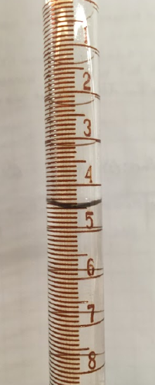
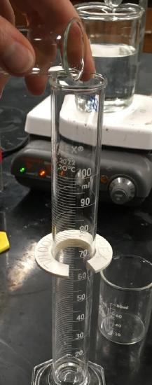
The numbers of measured quantities, unlike defined or directly counted quantities, are not exact. To measure the volume of liquid in a graduated cylinder, you should make a reading at the bottom of the meniscus, the lowest point on the curved surface of the liquid.
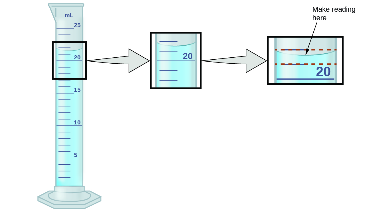
Refer to the illustration in Figure 01.1. The bottom of the meniscus in this case clearly lies between the 21 and 22 markings, meaning the liquid volume is certainly greater than 21 mL but less than 22 mL. The meniscus appears to be a bit closer to the 22-mL mark than to the 21-mL mark, and so a reasonable estimate of the liquid’s volume would be 21.6 mL. In the number 21.6, then, the digits 2 and 1 are certain, but the 6 is an estimate. Some people might estimate the meniscus position to be equally distant from each of the markings and estimate the tenth-place digit as 5, while others may think it to be even closer to the 22-mL mark and estimate this digit to be 7. Note that it would be pointless to attempt to estimate a digit for the hundredths place, given that the tenths-place digit is uncertain. In general, numerical scales such as the one on this graduated cylinder will permit measurements to one-tenth of the smallest scale division. The scale in this case has 1-mL divisions, and so volumes may be measured to the nearest 0.1 mL.
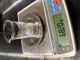
This concept holds true for all measurements, even if you do not actively make an estimate. If you place a quarter on a standard electronic balance, you may obtain a reading of 6.72 g. The digits 6 and 7 are certain, and the 2 indicates that the mass of the quarter is likely between 6.71 and 6.73 grams. The quarter weighs about 6.72 grams, with a nominal uncertainty in the measurement of ± 0.01 gram. If we weigh the quarter on a more sensitive balance, we may find that its mass is 6.723 g. This means its mass lies between 6.722 and 6.724 grams, an uncertainty of 0.001 gram. Every measurement has some uncertainty, which depends on the device used (and the user’s ability). All of the digits in a measurement, including the uncertain last digit, are called significant figures or significant digits. Note that zero may be a measured value; for example, if you stand on a scale that shows weight to the nearest pound and it shows “120,” then the 1 (hundreds), 2 (tens) and 0 (ones) are all significant (measured) values.
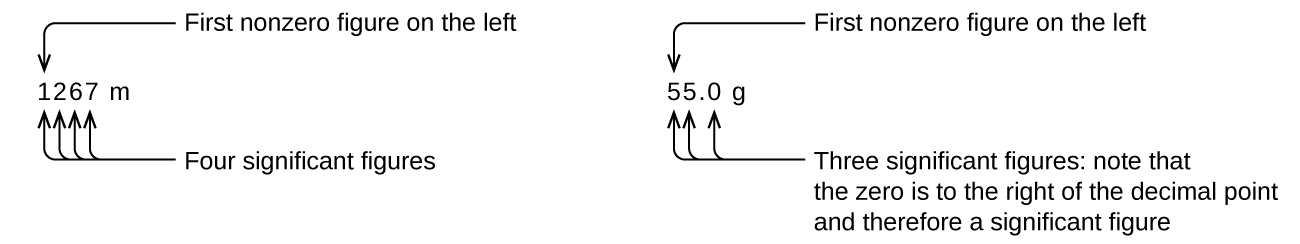
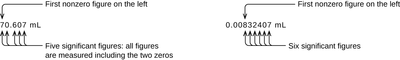
Whenever you make a measurement properly, all the digits in the result are significant. But what if you were analyzing a reported value and trying to determine what is significant and what is not? Well, for starters, all nonzero digits are significant, and it is only zeros that require some thought. We will use the terms “leading,” “trailing,” and “captive” for the zeros and will consider how to deal with them.
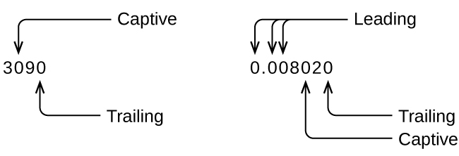
Starting with the first nonzero digit on the left, count this digit and all remaining digits to the right. This is the number of significant figures in the measurement unless the last digit is a trailing zero lying to the left of the decimal point.
Captive zeros result from measurement and are therefore always significant. Leading zeros, however, are never significant—they merely tell us where the decimal point is located.
The leading zeros in this example are not significant. We could use exponential notation (as described in Appendix B) and express the number as 8.32407 × 10⁻³; then the number 8.32407 contains all of the significant figures, and 10−3 locates the decimal point.
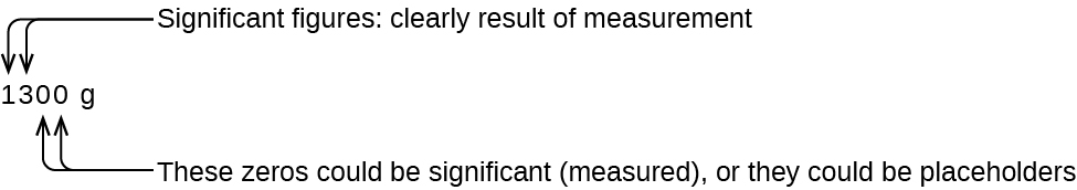
The number of significant figures is uncertain in a number that ends with a zero to the left of the decimal point location. The zeros in the measurement 1,300 grams could be significant or they could simply indicate where the decimal point is located. The ambiguity can be resolved with the use of exponential notation: 1.3 ×× 103 (two significant figures), 1.30 × 10³ (three significant figures, if the tens place was measured), or 1.300 × 10³ (four significant figures, if the ones place was also measured). In cases where only the decimal-formatted number is available, it is prudent to assume that all trailing zeros are not significant.
When determining significant figures, be sure to pay attention to reported values and think about the measurement and significant figures in terms of what is reasonable or likely—that is, whether the value makes sense. For example, the official January 2014 census reported the resident population of the US as 317,297,725. Do you think the US population was correctly determined to the reported nine significant figures, that is, to the exact number of people? People are constantly being born, dying, or moving into or out of the country, and assumptions are made to account for the large number of people who are not actually counted. Because of these uncertainties, it might be more reasonable to expect that we know the population to within perhaps a million or so, in which case the population should be reported as 317 million, or 3.17×10⁸ people.
Significant Figures in Calculations
A second important principle of uncertainty is that results calculated from a measurement are at least as uncertain as the measurement itself. We must take the uncertainty in our measurements into account to avoid misrepresenting the uncertainty in calculated results. One way to do this is to report the result of a calculation with the correct number of significant figures, which is determined by the following three rules for rounding numbers:
- When we add or subtract numbers, we should round the result to the same number of decimal places as the number with the least number of decimal places (the least precise value in terms of addition and subtraction).
- When we multiply or divide numbers, we should round the result to the same number of digits as the number with the least number of significant figures (the least precise value in terms of multiplication and division).
- If the digit to be dropped (the one immediately to the right of the digit to be retained) is less than 5, we “round down” and leave the retained digit unchanged; if it is more than 5, we “round up” and increase the retained digit by 1; if the dropped digit is 5, we round up or down, whichever yields an even value for the retained digit. (The last part of this rule may strike you as a bit odd, but it’s based on reliable statistics and is aimed at avoiding any bias when dropping the digit “5,” since it is equally close to both possible values of the retained digit.)
The following examples illustrate the application of this rule in rounding a few different numbers to three significant figures:
- 0.028675 rounds “up” to 0.0287 (the dropped digit, 7, is greater than 5)
- 18.3384 rounds “down” to 18.3 (the dropped digit, 3, is less than 5)
- 6.8752 rounds “up” to 6.88 (the dropped digit is 5, and the retained digit is even)
- 92.85 rounds “down” to 92.8 (the dropped digit is 5, and the retained digit is even)
Pre Lab Video
Procedure
Buret:
Step 1
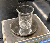
 Clean and dry a 100 mL beaker. Weigh the beaker. Note: You should use the same balance every time in this experiment. Record the mass of your beaker.
Step 2
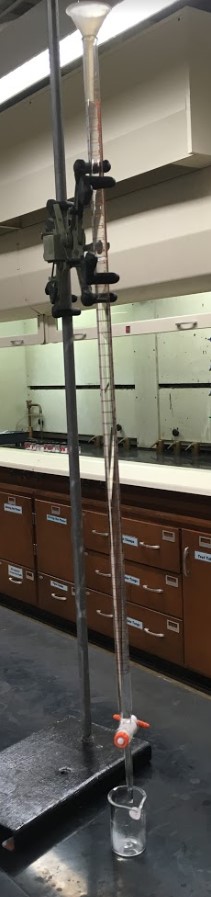 Fill the buret to approximately 0 mL with sodium chloride solution. You do not need to have it exactly at 0.00mL, but somewhere close and below the mark.
Step 3
 Open the stop cock and allow it to fill with solution. Read the volume and record this as the initial volume (remember to read correct number of significant figures).
Step 4
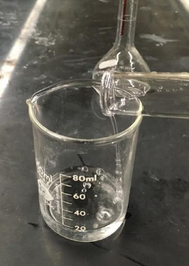
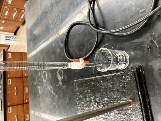 Allow approximately 15 mL of your sodium chloride solution sample into the pre-weighed beaker. Record the volume as the final volume. Note: burets are read from top down, so the value should be somewhere around 15.
Step 5
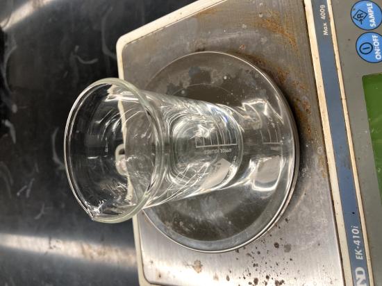
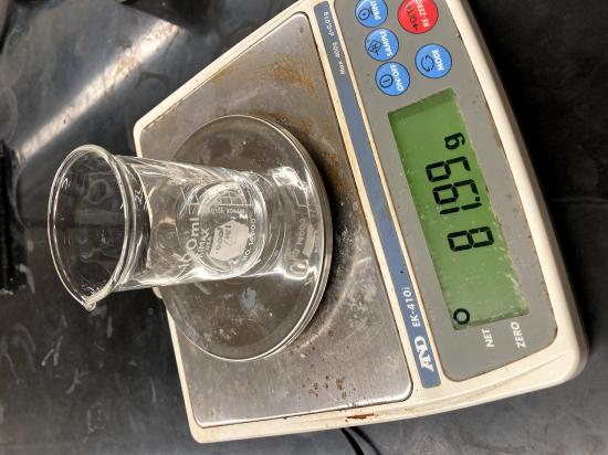 Weigh the beaker and solution. Record the mass.
Step 6
 Leaving the sodium chloride solution that you just measured in the beaker, dispense approximately 15 mL more solution into the beaker using your buret, being sure to record the initial and final volumes. Again, the final volume should have a value around 30. DO NOT REFILL THE BURET. Reweigh the beaker and sodium chloride solution. Record its mass in your notebook.
Step 7
Repeat step 3 so that you have three data points. Dispose of the sodium chloride solution sample down the drain.
Graduated Cylinder:
Step 1
 Dry your beaker and reweigh it, being sure to record the mass in your notebook. Do not assume the mass is the same as before.
Step 2
 Measure approximately 15 mL of your sodium chloride solution in a 100 mL graduated cylinder. Read the volume to the correct number of significant figures and record it in your notebook.
Step 3
 Pour the sodium chloride solution into your beaker and weigh the beaker and solution together. Record the mass in your notebook.
Step 4
 Leaving the sodium chloride solution you just measured in the beaker, repeat steps 2 and 3 twice more.
Calculations:
Step 1
Make a table of your data. You should have three measurements of sodium chloride solution and beaker using the buret and the graduated cylinder.
Step 2
Calculate (using the correct number of significant figures) the mass of sodium chloride solution added in each step.
Step 3
Calculate (using the correct number of significant figures) the density of sodium chloride solution using the equation
\[D = \frac{m}{V} \label{2}\]
where m=mass in grams and V=volume in mL
Step 4
Do this for each measurement that you made and using your exchanged data. You should have 6 density measurements.
How does the density you measured compare to that of water?
Graphing Practice:
Part 1:
You are given the following results from a sample carbon dioxide gas under standard pressure (1atm).
| Volume (L) | Temperature (oC) |
| 24.7 | 35.49 |
| 32.1 | 91.72 |
| 34.8 | 149.95 |
| 40.6 | 218.51 |
| 46.2 | 281.51 |
| 50.3 | 331.88 |
You also want to know the volume at two other temperatures but were unable to obtain this data directly from the experiment. These temperatures are 220 oC and 335 oC.
Step 1
Make a graph in Excel using the volume and temperature data, including the equation and the R2 value. See directions below. Make one graph choosing a trendline that is linear and print a copy. Make a second graph using the data but now choose a trendline that is an exponential fit. Finally, make a third graph with the data and choose a power trend line. Be sure to print copies of all three graphs. Based on the R2 value which trendline gives the best fit?
Step 2
Using the best curve provided by Excel and the equation on the graph, what is the volume of product at 220 oC, at 335 oC?
Part 2:
The following are results from an experimental determination of the volume of nitrogen at various pressures at room temperature (298 K).
| Volume (mL) | Pressure (atm) |
| 41.6 | 0.526 |
| 32.7 | 0.658 |
| 26.2 | 0.789 |
| 24.3 | 0.921 |
| 21.6 | 1.053 |
| 18.9 | 1.184 |
| 17.4 | 1.316 |
| 15.6 | 1.447 |
| 13.9 | 1.579 |
Step 1
Graph this data using Excel. Try several trendlines and print the best version. How does this graph compare with the best graph for Part A? Explain your observations.
Step 2
What would your volume be at a pressure of 1.400 atm? 2.100 atm?
Part 3:
Step 1
Using your data, create a graph plotting the mass vs. volume for both the buret data and the graduated cylinder data. Be sure to use the total volumes and masses for each run. Please choose a linear trendline.
Step 2
Given the equation, what does the slope of the line represent?